Congratulations, you made it through your first neural networks lab! What we built was already pretty cool, even the test set classification performance wasn't that great. Don't worry, we really just scratched the surface of what neural nets can do! Let's see how we can extend neural networks even further.
You will be able to:
- Explain how you can extend the logistic regression neural network example to "deeper" neural network
- How to structure your data to build a neural network
- Know what activation functions are and which one to use where
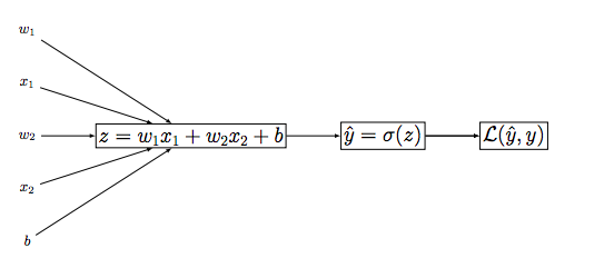
Let's look back at our logistic regression neural network example. In the image below, we represented what the forward propagation flow looks like. Now there is one important thing to notice, and that is that this logistic regression neural network is actually extremely shallow, as there are no hidden layers! How so?
In fact, what exactly does a neuron in a neural network do? The purpose of a neuron is 2-fold
- it transforms the inputs doing a linear transformation ( genre $ w x+b$)
- It uses an activation function (genre sigmoid, or another activation function. See more later)
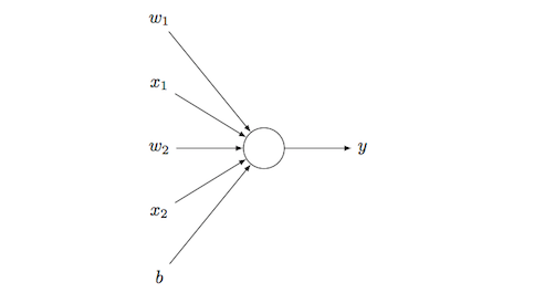
A more correct representation of the neural network is then as follows:
This means that there is only one neuron in the logistic regression neural network is basically a neuron in the output layer. It takes inputs that we know, and it directly outputs the observed output, with no layers in between. If this is the case, the neural network network is a 1-layer neural network.
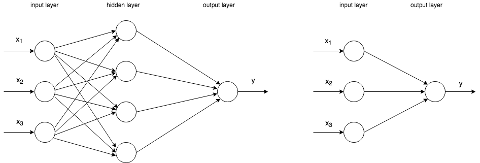
To make it even more clear, let's look at the network on the left below, which you might remember from the previous lecture. You can think of this network as a logistic regression-kind neural network, but with an extra layer plugged in with 4 nodes. This extra layer is a hidden layer, because we do not directly observe the output of this layer. This network is a 2-layer neural network, or a neural network with 1 hidden layer.
Why is this picture on the left hand side a 2-layer neural network? Don't we see 3 layers of nodes? Well, technically, the input layer is not a layer: no transformations happen here, it's simply a layer of inputs. That's why we included the example on the right hand side above. This is basically (again) another way of representing the logistic regression example, the same type of network as the one you've seen in the image right before. Sometimes the input layer will be denoted with actual nodes, sometimes it won't. Just remember that this layer does not count as an actual layer. When we refer to it, we'll say it's layer with index 0.
Let's look at this network going forward. With deeper networks, we'll need to introduce new notation. Generally, the output of layer
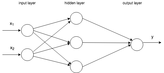
For our 2-layer neural network above, this means that:
-
$x = a^{[0]}$ as x is what comes out of the input layer - $a^{[1]} = \begin{bmatrix} a^{[1]}_1 \ a^{[1]}_2 \ a^{[1]}_3 \\end{bmatrix}$ is the value generated by the hidden layer
-
$\hat y = a^{[2]}$ , the output layer will generate a value$a^{[2]}$ , which is equal to$\hat y$ .
Rember that in each of the nodes in the hidden layer, a linear transformation will take place, as well as a transormation because of an activation function.
Let's look at the first node in the hidden layer. The linear transformation that takes place is $ z^{[1]}_1 = w^{[1]}_1 x +b^{[1]}_1$, and the activation
extending this to the two other nodes in the hidden layer, this gets us to the following equations for the hidden layer:
$ z^{[1]}_1 = w^{[1]}_1 x +b^{[1]}_1$ and
$ z^{[1]}_2 = w^{[1]}_2 x +b^{[1]}_2$ and
$ z^{[1]}_3 = w^{[1]}_3 x +b^{[1]}_3$ and
Now, let's discuss the dimensions of all these elements.
$w^{[1]} = \begin{bmatrix} w^{[1]}{1,1} & w^{[1]}{2,1} & w^{[1]}{3,1} \ w^{[1]}{1,2} & w^{[1]}{2,2} & w^{[1]}{3,2}\end{bmatrix}$
where, eg.
When multiplying the transposed (making it a 2 x 3 matrix) of this matrix
and add $b^{[1]} = \begin{bmatrix} b^{[1]}_1 \b^{[1]}_2 \ b^{[1]}_3 \end{bmatrix}$, we obtain $z^{[1]} = \begin{bmatrix} z^{[1]}_1 \z^{[1]}_2 \ z^{[1]}_3 \end{bmatrix}$. Similarly, we have $a^{[1]} = \begin{bmatrix} a^{[1]}_1 \a^{[1]}_2 \ a^{[1]}_3 \end{bmatrix}$ and corresponding sigmoid functions.
Now, let's try and move forward in our network. Recall that
$x = \begin{bmatrix} x_1 \x_2\end{bmatrix} \equiv a^{[0]}$ and that
Then, given input
Some questions to think about
- What are the dimensions of the matrices associated here?
- The 4 expressions above don't take into account several training samples. Imagine we use a superscript (i). How do you rewrite these epressions?
$z^{1} = w^{[1]T} a^{0} + b^{[0]}$
$z^{2} = w^{[2]T} a^{1} + b^{[2]}$
In the lab, you'll learn how to vectorize this!
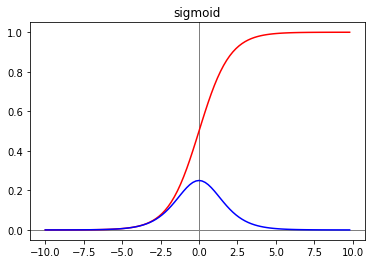
Until now, we've only discussed the sigmoid activation function. The sigmoid function is nearly always the go-to in the output layer of a binary classification problem, but in hidden layers, many other. In the code block below, you can find some functions we created so we can plot them below. Note that we plot the actual activation functions as well as their derivatives!
import numpy as np
import matplotlib.pyplot as plt

def sigmoid(x, derivative=False):
    f = 1 / (1 + np.exp(-x))
    if (derivative == True):
        return f * (1 - f)
    return f

def tanh(x, derivative=False):
    f = np.tanh(x)
    if (derivative == True):
        return (1 - (f ** 2))
    return np.tanh(x)

def relu(x, derivative=False):
    f = np.zeros(len(x))
    if (derivative == True):
        for i in range(0, len(x)):
            if x[i] > 0:
                f[i] = 1
            else:
                f[i] = 0
        return f
    for i in range(0, len(x)):
        if x[i] > 0:
            f[i] = x[i]
        else:
            f[i] = 0
    return f

def leaky_relu(x, leakage = 0.05, derivative=False):
    f = np.zeros(len(x))
    if (derivative == True):
        for i in range(0, len(x)):
            if x[i] > 0:
                f[i] = 1
            else:
                f[i] = leakage
        return f
    for i in range(0, len(x)):
        if x[i] > 0:
            f[i] = x[i]
        else:
            f[i] = x[i]* leakage
    return f

def arctan(x, derivative=False):
    if (derivative == True):
        return 1/(1+np.square(x))
    return np.arctan(x)

z = np.arange(-10,10,0.2)Let's have a look at the sigmoid again. Recall that the mathematical expression of the sigmoid is $ a=\dfrac{1}{1+ \exp(-z)}$, and this outputs activation values somewhere between 0 and 1.
y = sigmoid(z)
dy = sigmoid(z, derivative=True)
plt.title("sigmoid")
plt.axhline(color="gray", linewidth=1,)
plt.axvline(color="gray", linewidth=1,)
plt.plot(z, y, 'r')
plt.plot(z, dy, 'b')
[<matplotlib.lines.Line2D at 0x10ea11438>]
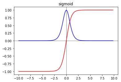
The hyperbolic tangent (or tanh) function goes between -1 and +1, and is in fact a shifted version of the sigmoid function, with formula $ a=\dfrac{\exp(z)- \exp(-z)}{\exp(z)+ \exp(-z)}$. For intermediate layers, the tanh function generally performs pretty well because, with values between -1 and +1, the means of the activations coming out are closer to zero!
y = tanh(z)
dy = tanh(z, derivative=True)
plt.title("sigmoid")
plt.axhline(color="gray", linewidth=1,)
plt.axvline(color="gray", linewidth=1,)
plt.plot(z, y, 'r')
plt.plot(z, dy, 'b')
[<matplotlib.lines.Line2D at 0x10ea77f98>]
A disadvantage of both tanh and sigmoid is that, when
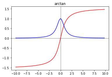
The inverse tangent (arctan) function has a lot of the same qualities that tanh has, but the range roughly goes from -1.6 to 1.6, and the slope is more gentle than the one we saw using the tanh function.
y = arctan(z)
dy = arctan(z, derivative = True)
plt.title("arctan")
plt.axhline(color="gray", linewidth=1,)
plt.axvline(color="gray", linewidth=1,)
plt.plot(z, y, 'r')
plt.plot(z, dy, 'b')
[<matplotlib.lines.Line2D at 0x10ebb67b8>]
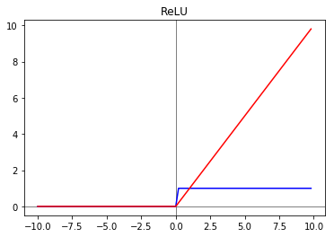
This is probably the most popular activation function, along with the tanh! The fact that the activation is exactly 0 when
plt.title("ReLU")
y = relu(z)
dy = relu(z, derivative=True)
plt.axhline(color="gray", linewidth=1,)
plt.axvline(color="gray", linewidth=1,)
plt.plot(z, dy, 'b')
plt.plot(z, y, 'r')
[<matplotlib.lines.Line2D at 0x10ec8b7b8>]
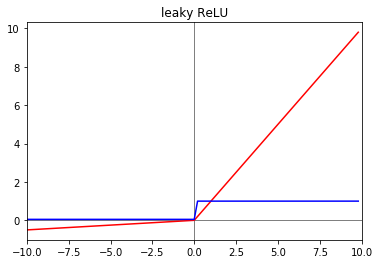
The leaky ReLU solves the derivative issue by allowing for the activation to be slightly negative when
# the default leakage here is 0.05!
y = leaky_relu(z)
dy = leaky_relu(z, derivative=True)
plt.axhline(color="gray", linewidth=1,)
plt.axvline(color="gray", linewidth=1,)
plt.title("leaky ReLU")
plt.xlim(-10,10)
plt.plot(z, y, 'r')
plt.plot(z, dy, 'b')
[<matplotlib.lines.Line2D at 0x10ed5a0b8>]
In this lecture, you obtained a better intuition on how "deeper" neural networks work, and you learned about some very important notation that will be used when building deeper networks. Additionally, you learned about activation functions other than the sigmoid function, and what their derivatives look like.
