frankiethull
why does this repo exist? To store some artsy rayshader examples with chaotic julia simulations. i.e. how to dual wield Julia & R to make beautiful graphics.
waveshading was tagged in a few playful posts on my Twitter/X. This related two systems: one in Julia, one in R.
Tested both Julia’s waterlily.jl and oceananigans.jl computational fluid dynamics engines which allow chaotic fluid simulations. “rayshader” is a 3d plotting toolkit in R. Combining the two langs’ libs mainly for funsies, trying out multiple esoteric open-source pkgs, & testing multilingual quarto documents. As an added layer, examples below use Arrow.jl to write the data, and arrow library in R to read in the data.
Marrying the two together (Julia + R) sparked a lot of interest (“let me see your code!”) type of requests on X. Not necessarily for scientific reasons, but for artistic renderings of fluids!
Below is a simple tutorial on running simulations in Julia and creating visualizations in R. Whether it be terrain-based, fluid flows, cloud physics, or whatever; there are a lot of cool artistic ways to leverage rayshader + various tools from Python or Julia to make some really cool renderings.
let’s run some code in julia, then pass the results to R. Below we are running a julia code-chunk.
Note, you can do any waterlily, oceananigans, or other julia example, but this one is short and requires less domain knowledge. https://docs.makie.org/stable/reference/plots/surface/
This example is borrowed from Makie documentation which seemed like a better start for a tutorial. Instead of going all out on a fluid simulation, we are going to simulate a single matrix. This is the best starting point imo!
# pkg setup for julia is pretty easy, example given:
# import Pkg; Pkg.add("package_name")

using SparseArrays
using LinearAlgebra
# using GLMakie


# This example was provided by Moritz Schauer (@mschauer).

# Define the precision matrix (inverse covariance matrix)
# for the Gaussian noise matrix.  It approximately coincides
# with the Laplacian of the 2d grid or the graph representing
# the neighborhood relation of pixels in the picture,
# https://en.wikipedia.org/wiki/Laplacian_matrix

function gridlaplacian(m, n)
    S = sparse(0.0I, n*m, n*m)
    linear = LinearIndices((1:m, 1:n))
    for i in 1:m
        for j in 1:n
            for (i2, j2) in ((i + 1, j), (i, j + 1))
                if i2 <= m && j2 <= n
                    S[linear[i, j], linear[i2, j2]] -= 1
                    S[linear[i2, j2], linear[i, j]] -= 1
                    S[linear[i, j], linear[i, j]] += 1
                    S[linear[i2, j2], linear[i2, j2]] += 1
                end
            end
        end
    end
    return S
end
gridlaplacian (generic function with 1 method)
# d is used to denote the size of the data
d = 150
150
 # Sample centered Gaussian noise with the right correlation by the method
 # based on the Cholesky decomposition of the precision matrix
data = 0.1randn(d,d) + reshape(
        cholesky(gridlaplacian(d,d) + 0.003I) \ randn(d*d),
        d, d
)
150×150 Matrix{Float64}:
-2.13805 -1.94965 -2.10359 … -5.97555 -5.73233 -6.00414
-1.02904 -1.04465 -1.68999 -5.93925 -5.84186 -5.79731
-1.61541 -0.856065 -1.9808 -5.97519 -6.11237 -5.64964
-1.57751 -1.39463 -1.7793 -5.04787 -4.80033 -5.20001
-0.833541 -0.917326 -0.860234 -4.56373 -4.87722 -5.36495
-0.544637 -0.580403 -1.63535 … -4.42889 -5.00575 -4.96543
-0.793416 -1.10866 -1.42821 -3.83051 -4.53027 -4.45252
-1.16538 -1.0411 -1.19002 -3.53441 -3.36568 -3.39797
-0.413468 -0.411806 -0.494561 -2.37381 -1.98162 -1.98826
0.642052 0.317184 0.25955 -1.45563 -1.00251 -0.929579
⋮ ⋱
0.284687 1.51012 1.63325 -14.042 -13.4928 -13.7777
0.534829 0.68485 0.599681 -13.6971 -14.1725 -14.2502
1.35339 1.43253 1.37181 -14.4908 -14.974 -14.841
1.42905 1.85022 2.04163 -15.3576 -15.3393 -15.2397
0.89054 1.24337 1.01869 … -15.3701 -14.9391 -14.4177
0.114869 0.149387 -0.173205 -15.5042 -15.1111 -14.7342
-1.11646 -0.191676 -0.892522 -14.6317 -14.7718 -15.1839
-2.48818 -2.00189 -1.59932 -14.4368 -15.5093 -16.5131
-3.22367 -2.81377 -2.71081 -15.6244 -15.7154 -16.6066
# makie code is commented out, instead we will pass the data to R for rayshader.
# surface(data; shading = NoShading, colormap = :deep)
# surface(data; shading = NoShading, colormap = :deep)
convert the matrix to dataframe and save it off as an arrow file for R
using Arrow
using DataFrames

laplace_df = DataFrame(data, :auto)
150×150 DataFrame
Row │ x1 x2 x3 x4 x5 x6 x7 ⋯
│ Float64 Float64 Float64 Float64 Float64 Float64 Floa ⋯
─────┼──────────────────────────────────────────────────────────────────────────
1 │ -2.13805 -1.94965 -2.10359 -2.48174 -2.42099 -2.67788 -4.0 ⋯
2 │ -1.02904 -1.04465 -1.68999 -2.11412 -2.44765 -3.29165 -4.1
3 │ -1.61541 -0.856065 -1.9808 -2.59396 -2.52635 -3.53037 -4.6
4 │ -1.57751 -1.39463 -1.7793 -2.81635 -3.41164 -3.8532 -4.5
5 │ -0.833541 -0.917326 -0.860234 -1.9965 -2.57298 -2.8754 -3.5 ⋯
6 │ -0.544637 -0.580403 -1.63535 -1.68791 -1.57463 -1.79414 -1.9
7 │ -0.793416 -1.10866 -1.42821 -1.86227 -1.76905 -1.69462 -1.8
8 │ -1.16538 -1.0411 -1.19002 -1.13643 -0.787755 -0.407784 -0.8
⋮ │ ⋮ ⋮ ⋮ ⋮ ⋮ ⋮ ⋱
144 │ 1.35339 1.43253 1.37181 1.74211 2.0665 3.00317 3.3 ⋯
145 │ 1.42905 1.85022 2.04163 1.33177 1.77917 2.20661 3.0
146 │ 0.89054 1.24337 1.01869 0.909277 1.36002 0.977153 1.7
147 │ 0.114869 0.149387 -0.173205 -0.191221 -0.261122 -0.414318 0.2
148 │ -1.11646 -0.191676 -0.892522 -0.325694 -0.94129 -1.13833 -0.4 ⋯
149 │ -2.48818 -2.00189 -1.59932 -1.85026 -1.5952 -1.69063 -0.9
150 │ -3.22367 -2.81377 -2.71081 -1.97549 -2.05071 -2.14482 -1.2
144 columns and 135 rows omitted
Arrow.write("laplacian.arrow", laplace_df)"laplacian.arrow"
next lets get the data setup in R for rayshader. There are a few ways to do this. First load the df into a data.frame, then create an id for each row-column and stretch it so it’s in a long format.
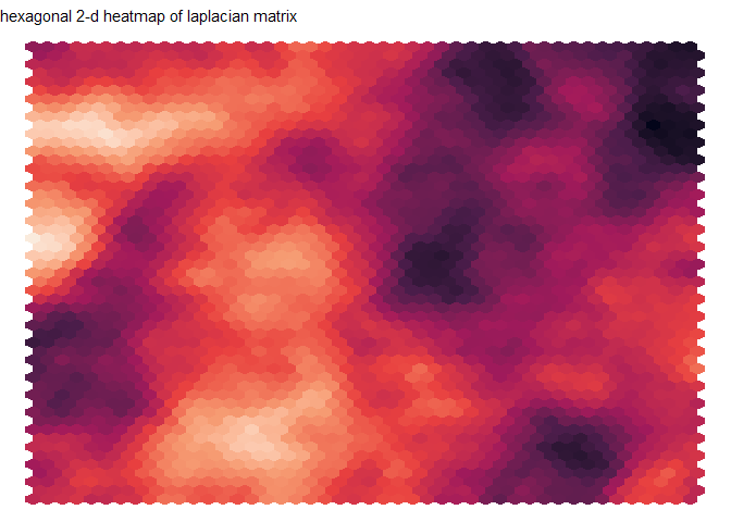
This will give us a lot of flexibility as we are going to use ggplot2 then convert the ggplot2 into a rayshader plot (if you are familiar with ggplot2, this is a shortcut).
From there, xy binning to approximate the density of the surface (makes a better visual imo). & 2-d hexagon bins work well.
library(dplyr)Attaching package: 'dplyr'
The following objects are masked from 'package:stats':
filter, lag
The following objects are masked from 'package:base':
intersect, setdiff, setequal, union
library(tidyr)
library(ggplot2)
Warning: package 'ggplot2' was built under R version 4.3.2
library(rayshader)

# julia output
laplace_df <- arrow::read_ipc_file("laplacian.arrow")

# let's get this xy-matrix into a long df:
laplace_long_df <- laplace_df |>
                   mutate(
                     x_id = row_number()
                   ) |>
                    tidyr::pivot_longer(-x_id, names_to = "y_id", values_to = "z") |>
                    mutate(
                      y_id = gsub("x", "", y_id),
                      y_id = as.numeric(y_id)
                    )

# ggplot hex display:
gg <-
laplace_long_df |>
    ggplot(aes(x = x_id, y = y_id, z = z)) +
  stat_summary_hex(fun = function(x) mean(x), bins = 45)  +
  scale_fill_viridis_c(option = 12) +
  theme_void() +
  theme(legend.position = "none")

gg + labs(subtitle = "hexagonal 2-d heatmap of laplacian matrix")
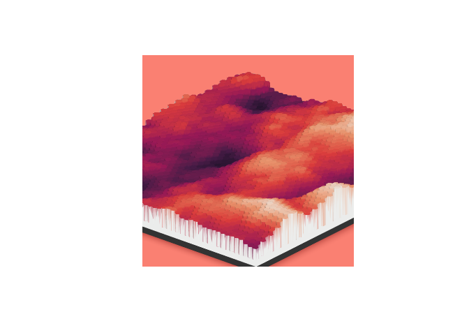
creating the 3D-ified ggplot with rayshader:
plot_gg(gg, height=5, width=4.5,
        phi   = 25,
        zoom  = 0.4,
        theta = -140,
        background = "salmon")

render_snapshot(filename = "rayshader_v1.png")
display the snapshot:
magick::image_read("rayshader_v1.png") |>
  plot()
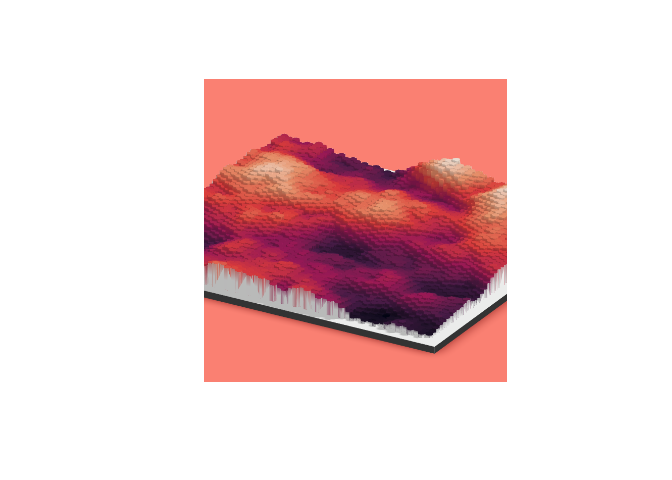
adjusting phi, theta, and zoom:
plot_gg(gg, height=5, width=4.5,
        phi   = 25,
        zoom  = 0.5,
        theta = 120,
        background = "salmon")

render_snapshot(filename = "rayshader_v2.png")

magick::image_read("rayshader_v2.png") |>
  plot()
from there, you can stitch multiple images together (if you have a delta such as time or some other step function you are iterating over. Like rotating phi or theta in a loop). If there are more than one file, create a video from a list of saved png files like so:
fps <- 10
av::av_encode_video(file_list, ‘output.mp4’, framerate = fps)
utils::browseURL(‘output.mp4’)
based on feedback will save off more complicated examples in an example subfolder. But think this is the best starting point for running CFD in Julia and shaders in R.
To recreate the original Twitter post, see this example:
https://clima.github.io/OceananigansDocumentation/stable/literated/convecting_plankton/
original post:
https://x.com/frankiethull/status/1744557482779742514?t=sgeF2vulucLE1h-xD9LJ1A&s=19
Additional notes:
my system has both julia and R installed on a windows machine. I have
RCall installed on Julia and JuliaCall installed on R. Julia is on my
env paths and this was ran using knitr via R, not a Julia Jupyter
kernel.


