Overview

The lime-plotter application plots data collected from robots in the First Robotics Competitions and plots them to the screen or to a PNG file. It can read data from CSV based log files, or via a networktables server (IE, from a robot over its wireless network).

Usage

Installation

Install any needed modules and the lime-plotter itself:

pip3 install --user --upgrade frc1678-lime-plotter

Things to plot are specified either via complex command line arguments with the -p switch, or via easier-to-read-and-write YAML configuration files (see the example below).

Datasources and loaders

There are a number of ways where lime-plotter can get data from in order to draw on its map:

CSV log files
The robot's Network Tables broadcasting
SVG files
Timers

Some of these data-sources (CSV and robot data) are specified on the command line, and others are part of the plot specification file (svg graphics and timers).

Reading from CSV log files

lime-plotter can be run with a -L switch to load CSV files from a file, multiple files, or a directory of files.

For example, to load a CSV file:

lime-plotter -L log.csv

Or calling it with a directory will try to get it to load all the files from a directory:

lime-plotter -L DIR

Table names will be assumed from the CSV file names.

Reading from Robot's FRC network tables

To continuously download data from a robot's broadcasted network tables, use the -N switch to specify the robot's IP address to connect to, and optionally a -T switch to specify a default table to read from.

lime-plotter -N 10.0.0.1 -T nettable

(in general, the -T switch shouldn't be needed except in rare cases)

Listing available tables / columns from the robot

In order to list the available variables that can be plotted, you can ask lime-plotter to list the variables it can find given the data source. This is most helpful when getting information from a robot, but also works with CSV logs. Here's an example of getting the list of current broadcasted variables from the robot:

lime-plotter -N 10.0.0.1 -l

Configuration documentation

Configuration files for lime-plotter are stored in YAML formatted configuration files. All data in a YAML file must be contained in a plots dictionary keyword, with each sub-keyword being the name of a plot. Within each plot should be an array of things to plot.

further details TBD -- see examples for now

Example configuration

The following are YAML file configuration examples.

Also see a complete example in example-configs/2021-example.yml

Example single graph

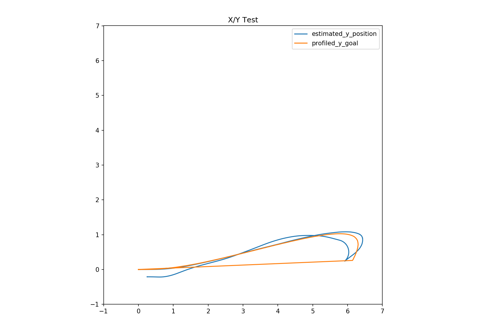
The following example configuration file specifies a single plot called position and plots two overlayed graphs from the Robot's datasets:

plots:
  position:
    - x: estimated_x_position
      y: estimated_y_position
      xmax: 7
      xmin: -7
      ymax: 7
      ymin: -7
      fixedAspect: True
      title: X/Y Test
    - x: profiled_x_goal
      y: profiled_y_goal
      table: drivetrain_status
      # limits the plot to the last 100 points
      last: 100

Saving this configuration to xy.yml and running lime-plotter to load logs from a log directory as follows:

lime-plotter -L log -y xy.yml -o xytest.png

Might produce the following graph:

Example multiple graphs

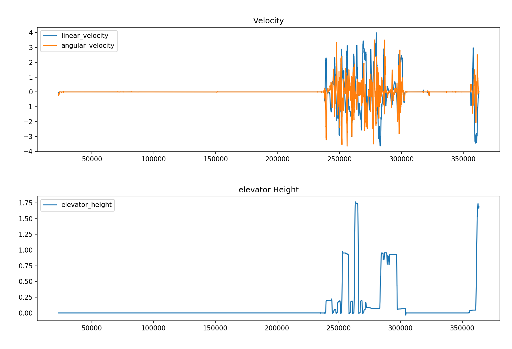
To display multiple plots, configuration files can contain multiple named entries.

plots:
  velocity:
    - y: linear_velocity
    - y: angular_velocity
      title: Velocity
  elevator:
    - y: elevator_height
      title: elevator Height

And run with

lime-plotter -L log -y multiple.yml -o multiple.yng

Will produce a graph similar to the following:

Plotting only a single plot from a config file

Note: you can use the -Y flag to plot only a selected set of sections of the YAML file. EG lime-plotter -L log -y multiple.yml -Y velocity will plot only the first graph.

Including an svg image (such as a field map)

Indicating that a plot is actually a static SVG file to be used as a background, set the plot's data_source to svg inside a plot:

plots:
  - data_source: svg
    file: 2020map.svg
    xmax: 629.25 # scale svg to these dimensions
    ymax: 323.25 # (2020 dimensions in inches)
    alpha: .5

In general, the SVG plotter is not a full featured SVG but can plot basic SVG lines. Anything else likely won't work.

As an example, here's a copy of the FRC 2020 map as a plottable SVG:

Including built in maps

The following map file names can be specified without actually having a file present, as they're included in the package data:

2021.svg
2020map.svg (just the playing field)
2020map-rev.svg (reverses the playing field top to bottom)
2020map-full.svg (the full field with human areas)
2019map.svg

adding offsets for your robot's starting position

When your robot starts at a point in the field, you can adjust it's xoff and yoff values to set the offsets into the field, with 0,0 being in the bottom left.

plots:
  position:
    - x: Robot X
      y: Robot Y
      xoff: 100
      yoff: 50
      fixedAspect: true

Animation

When plotting from networktables (-N) or with the -a switch applied, a window will open that will animate the data flowing over time (live in the case of networktables). You can use the -f switch to change the frame rate (when graphing CSV files, it'll draw faster with higher values -- the default is 20; when drawing from network tables it'll use this value as the polling frequency, and should be set to the same number of milliseconds that the robot is using to update tables).

Time markers

A final datasource is "time markers", which draws a small numbered circle every N seconds. It is configured like follows to add position annotations to an existing plot:

plots:
  timemarkers:
    # plot the regular robot x/y coordinates
    - x: Robot X
      y: Robot Y
      fixedAspect: true

    # Plot a larger (size 20) dot every 1 second ontop the Robot X/Y marks
    - data_source: timer
      marker_size: 20
      x: Robot X
      y: Robot Y
      delta: 1

Notes on operating system support:

Note on linux:

The default install path is ~/.local/bin/; make sure that's in your path or you can call it from there using ~/.local/bin/lime-plotter.

Notes on windows:

Windows installs python scripts differently. The executable is lime-plotter.exe and is located in c:\Users\YOU\AppData\Roaming\Python\Python37\Scripts\lime-plotter.exe

Notes on OSX:

It too has a special path -- watch the output of pip3 install to see where it gets installed and either call it with the full path name or put that directory in your path.

Running the code from the lime-plotter code repo

If you clone the lime-plotter repo to run the latest and greatest that isn't installable yet, this command should get you started:

PYTHONPATH=. python3 frc1678/limeplotter/main.py -y ../lime-plotter-config/mapped.yml

frc1678/lime-plotter