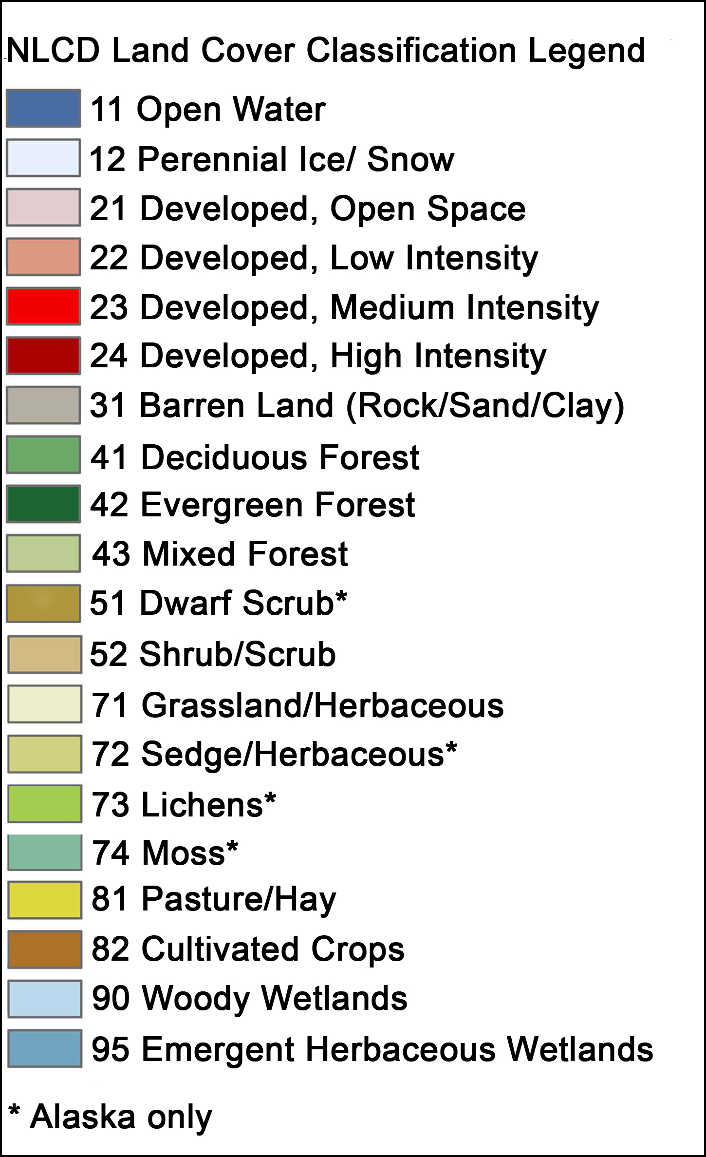
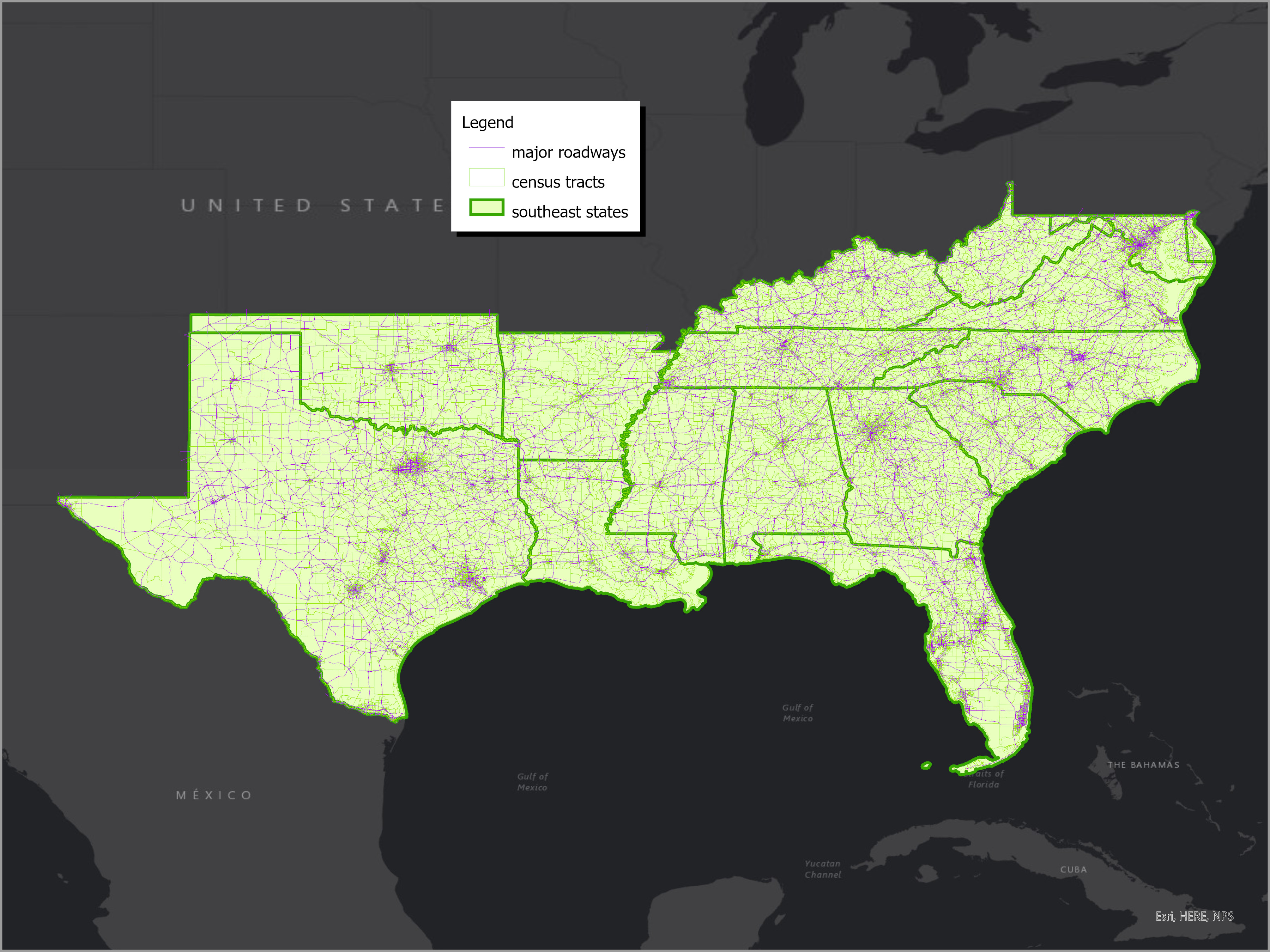
This is the project summary page for my ITCS 8190 course project. In this project, I succeeded in conducting multiple linear regression in a Hadoop / Apache Spark cluster running on Google Cloud Platform. My project was the application of regression towards predicting urban growth based on land cover and census demographic data. The unit of analysis is census tracts. Data for this project was retrieved from the US Census Bureau and the Multi-Resolution Land Characteristics (MRLC) Consortium. My presentation has been attached below in the Appendix.
-
Context: I chose to use my course project as an opportunity to learn more about Apache Spark and statistics and their interaction with geospatial research. I am a Ph.D. student in the Department of Geography at UNC Charlotte taking an advanced computer science course (ITCS 8190) because I want to bring computer science methods to Geographic Information Science (GIS). My background before GIS was web development as a computer science undergraduate at UNC Charlotte. I felt this project would be an easy introduction to the intersection of cloud computing and GIS, but was surprised and overwhelmed by the complexity involved. While I have learned a weighty tome of information about cloud computing this semester, I still have a lot of work ahead to understand the entire scope of this exciting topic.
-
Interesting: The most interesting aspect of this project is the distributed prediction of a multiple linear regression model using Apache Spark. Also of interest is the data preparation incorporating land cover and demographic data. I attempted to predict growth by using 2011 data for my independent variables, and 2016 data for my dependent variables. My line of thinking was that I could map indicators of future growth (population, roads, landcover) to an increase seen later in landcover.
In this course project, I used multiple linear regression to model urban growth. The model formula is:
Urban = Beta_0 + Beta_1*roadDens + Beta_2*popDens + Beta_3*barren + Beta_4*water + Beta_5*nature + Beta_6*agric

Where
  Urban  = Dependent variable, percent of census tract's land cover urban
  Beta_0 = Y-intercept coefficient
  Beta_{1..6} = Coefficients
  roadDens = (Length of roads in meters / area of tract in square meters)
  popDens = (ACS Estimated population / area of tract in square meters)
  barren = (NLCD Barren landcover pixels / total pixels in census tract)
  water = (NLCD Open Water landcover pixels / total pixels in census tract)
  nature = ((Forest + Shrub + Grassland + Wetlands) landcover pixels / total pixels in census tract)
  agric = ((Pasture + Crops) landcover pixels / total pixels in census tract)
I used the Google Cloud Platform Dataproc service to host a Hadoop cluster. This service has multiple images for cluster VM nodes. I chose Dataproc 1.5, which includes Ubuntu 18.04 LTS, Hadoop 2.10, and Spark 2.4. It also runs Python 3, which was my primary motivation for choosing this image.
- US Census American Community Survey
- Census tracts (with geometry). 5-year estimates of population Variable: B01003_001. Years: 2011, 2013, 2016. Num Features: 78,147 Size: 349MB
- US Census TIGER/LINE Shapefiles
- Primary and Secondary Roads (geometry). Years: 2011, 2013, 2016. Num Features: (159,266 141,574 141,041) respectively. Size: 809MB
- National Land Cover Database
- Raster image datasets (30 meter by 30 meter resolution). Years: 2011, 2013, 2016. Size: 60GB
- Download Census data for years 2011, 2013, 2016
- Population Estimate from American Community Survey (5-Year)
- TIGER/LINE Roads
- Save to disk as ESRI Shapefiles
- Calculate road density per census tract
- ST_INTERSECTION: Cut road lines with tract polygon edges
- Calculate lengths of road line segments
- Calculate area of census tracts
- Group By tract ID and sum all segment lengths
- Divide summed lengths by tract areas to get density
- (Therefore, tract size no longer matters)
- Calculate population density per census tract
- Left Join road density data frame with population data frame (to re-use census tract area column)
- Divide population estimate by tract area
- Rename columns for convenience
- Write population and road densities to CSV
- Test Linear Regression in R
- By suggestion of the instructor, it was very useful to have known-valid values to validate my implementation later in Apache Spark.
cc.fit.2011 = glm(urbany ~ roaddens + popdens + barren + water + nature + agric , data = lcpr2011)
- Upload data to Hadoop HDFS
freezurbern@cluster-95c6-m:/home/ubuntu$ hadoop fs -put lcpr2011.csv /user/root/lcpr2011.csvfreezurbern@cluster-95c6-m:/home/ubuntu$ hadoop fs -put lcpr2013.csv /user/root/lcpr2013.csv- For Google Dataproc, upload the files following their tutorial
- Run model using independent variables from 2011 and dependent variable from 2016
- Predict using independent variables from 2013 and dependent variable from 2016
- Data Loading
- After uploading to HDFS, using spark to read CSV
- Cleanup data columns and rename
- Compute multiple linear regression coefficients
- Based on my Assignment 2 code
- Store the coefficients on HDFS for later use
- Distributed prediction
- Loading new data from HDFS
- Loading coefficients from HDFS
- Adding coefficients as columns
- Computing dependent variable
- Return DataFrame with input data and prediction
- Data Export
- Saving computed prediction to HDFS
- Calculate R-squared
- Searching and Plotting
- Install geopandas on the Dataproc JupyterLab instance
- Upload Census polygons to Google Cloud Storage bucket
- Access bucket to load from shapefile
- Plot!
In this project, I further developed my knowledge of R to create my data pipeline. I chose R for this task because I am using it in another course this semester, and there are two very convienent packages authored by Kyle Walker:
These packages were instrumental in gathering Census data. Tidycensus is a convenient alternative to data.census.gov and tigris is a similar package for spatial data from the US Census. I utilized R Studio Server in a Docker container for reproducibile environments. Please see Appendix item 3 below for the Docker Compose script.
Another software essential to this project was ESRI's ArcGIS Pro. I used ArcGIS to tabulate raster image pixels by census tracts. This converted raster image data to counts of pixels as a CSV file.
These maps are plots from GeoPandas after joining the prediction output with census tract polygons. They were generated on a single node on the cluster. While not distributed, they provide a non-scientific visual cue of prediction results. One can compare my map outputs to the
US Population from the Census
to find I was able to accurately model urban areas. The map looks as expected, higher values at urban areas:
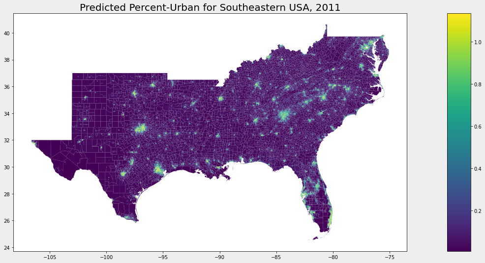
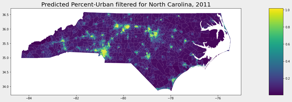
I also wanted to check if there was variation in my prediction results based on population or landcover. For example, are my predictions less accurate in extremely rural areas? To test this visually, I plotted the difference between actual and predicted (c16p11['diff'] = c16p11['urbany'] - c16p11['cy'] ):
Also included is a Pandas DataFrame with the actual column urbany and the predicted column cy:
- Manual calculation: I evaluated the performance of my linear regression model first by manually calculating a prediction:
betas = [0.9828573112718250737174230, 0.6322003963821229977071425, 4.0829155870278501794246040,
         0.0187037366133609578300323,-0.9753240641474236749530746,-0.9734866562156101466030123,
         -0.9760581738234358484262998]
ex_feature = ['01003010500',
              0.0093421030,
              0.0002470766835,
              0.01558030241,
              0.00715161422,
              0.501277074,
              0.08065999183,
              0.41091132]

ex_y = ex_feature[7]
ex_x = ex_feature[1:8]
calc = beta[0] + (beta[1]*ex_x[0]) + (beta[2]*ex_x[1]) + (beta[3]*ex_x[2]) + (beta[4]*ex_x[3]) + (beta[5]*ex_x[4]) + (beta[6]*ex_x[5])
print(calc)
# 0.41637306722808143
print(calc - ex_y)
# 0.005461747228081404
The result of this calculation is approximately +0.005, which shows my model overestimates the percent-urban by 0.5%. I find this result adequate but not inspiring, because 0.05% of a census tract (average size in my dataset is 2,436 acres) is 121 acres.
- R-Squared: I also implemented R-squared to calculate the goodness-of-fit of my prediction to my actual values. For 2011 data, I have an R-squared value of
0.9831. R-squared represents the percent of variance captured by the model out of the total variance. A value of 0.98 is a pleasant surprise, given my inexperience with Spark.
I have included a limited code snippet of calculating R-squared:
# calculate (y - yhat) ^2
def dfM(v,m):
    return math.pow((v - m), 2)
uDFM = udf(dfM, DoubleType())

def calcRsquared(inDATAFRAME):
    # Calculate means
    df_stats = dfPred.select(
        _mean(col('urbany')).alias('ymean'),
        [...]
    ).collect()
    # Add means as columns
    tmpr2 = (dfPred.withColumn("ymean", lit(ymean))
                   [...])

    # Calc dist from means
    tmpr2_ym = (tmpr2.withColumn("ymdist", uDFM('urbany', 'ymean'))
                     [...])

    r2_stats = tmpr2_ym.select(
        _sum(col('yhmdist')).alias('numer'),
        [...]
    ).collect()

    # divide actual y-value mean by lin reg estimated y-value mean
    rsquared = [...]['numer'] / [...]['denom']

    print(f"R-Squared is {rsquared}")
return rsquared ✔️ Loading my data into Apache Spark
- Please refer to the Python files in my CANVAS submission
✔️ Analyze the South East region of the United States
- See Appendix 2 at the end of this page for a map of states, census tracts, and major roadways
✔️ Implementing multiple linear regression in Apache Spark
- See Apache Spark section above
✔️ Train a model
- See Apache Spark section above
✔️ Predict urban growth
- See Results section above
✔️ Export and map the predicted urban growth
- See Results section above
❌ Use data across the entire United States
- I did not accomplish this likely goal due to pre-processing time associated with road density. Calculating density for the southeastern United States took atleast 30 minutes depending on which machine was running the R code. With more time, I believe I could expand my analysis.
❌ Import my datasets directly into spark without preprocessing in R or ArcGIS Pro
- I did not accomplish this stretch-goal because Apache Spark does not have native support for raster image data, and my knowledge of the platform is not yet advanced enough to implement this myself.
✔️ Distributed prediction using Spark DataFrames
✔️ Running my code on a Google Cloud Platform cluster
✔️ Loading data from a Google Cloud Storage Bucket
✔️ Documenting projects on GitHub Pages
Briefly, here are the challenges encountered during this project.
- My project proposal described my unit of analysis as a raster image pixel. This was ultimately impractical due to Apache Spark's affinity for matricies and tables. With the gracious permission of the instructor, I was able to move to census tracts as my primary unit. Census tracts are given a unique GEOID primary key by the Census which is consistent through time and datasets.
- My second error in my project proposal was defining my research question and approach. I intended to implement logistic regression on Apache Spark to determine whether an area had experienced urban growth or not. After digging into the datasets, I found my urban variable was continuous between 0.0 and 1.0. I contacted the instructor who again allowed me to modify my project to work around this mistake.
- Another issue I encountered was moving from local Spark development in a Jupyter Notebook to JupyterLab in the cloud. Not only was the storage medium different (local disk versus HDFS), commands took much longer to start executing in the cloud. While my development pace was slowed by working in the cloud, I knew my code would work there because I could debug as I developed my scripts, not afterwards.
- This project demonstrated I have much to learn about linear algebra, matrices, and algorithms. I believe most of my mistakes in this course were due to my lack of understanding about the mathematics behind techniques covered. I expect to further my understanding in later courses focused on these statistical topics.
-
My first lesson learned was that much preparation must go into a project proposal. My challenges were a result of too little data exploration and knowledge of methods. In the future, I will consider datasets carefully and properly document the exact columns of each dataset used in my proposed analysis.
-
Data pipelines with multiple tools on multiple machines should be avoided. For this project, I used R Studio in a Docker container on my server to conduct preprocessing of census data and later for processing of ArcGIS output. Census tract polygons were copied from R Studio to ArcGIS Pro on my laptop for tabulation with land cover raster images. Then, the tabulations were copied back to R Studio for additional analysis. This back-and-forth between multiple machines and multiple applications should be avoided if possible. A purely-Spark data pipeline would have been even cleaner.
-
Native libraries are a convenient black box with detailed outputs. By implementing regression by-hand, I learned exactly what is going on behind the scenes of native functions. I also learned how much work is put into them to give useful outputs such as r-squared or RMSE.
- A job-gone-wrong can crash a Google Dataproc cluster. I painfully learned this lesson by asking for too much data to be returned in a Jupyter Notebook running on the single master node. Required rebooting the nodes.
-
Store code separately from data in the cloud. This is related to the previous lesson. One should store code separately (i.e. no code in HDFS!) in a place safe from cluster crashes. One should be able to completely re-initialize a cluster from scratch and lose no progress on their data analysis.
-
Split data within the same year In this project, I split my training and testing data by year (2011 and 2013) instead of within the same years. The professor made an excellent point that I'm being unfair to this model by training on 2011 and testing on 2013 when I should have used an 80%/20% train/test spplit within a year. I have used this method in previous experiences with machine learning, but did not realize it would be useful for multiple linear regression as well. I will look into this using Spark's 'sample' function.
- Introduction to multiple regression
- This resource was used to better understand the multiple linear regression problem as well as to serve as an example in R language
- PySpark Cheatsheet
- Spark on Google Cloud Platform
- Documenting using Markdown
- Calculating R Squared
Access is provided at http://YOUR_IP:8787
version: "3.7"
services:
  rocker:
    image: rocker/geospatial:4.0.2
    container_name: rocker
    restart: "no"
    ports:
      - "8888:8888"
      - "8484:8484"
      - "8787:8787"
    environment:
    - ROOT=TRUE
    - PASSWORD=rocker
    - DISABLE_AUTH=true
    - USERID=1000
    - GROUPID=1000
    - UMASK=022
    volumes:
    - /opt/cc-rstudio/rnb:/home/rstudio/rnb
This PDF includes fixes suggested by the professor, including documenting from which year each column comes from. Revised Presentation PDF


