A CFD Tutorial in Julia
A CFD Tutorial in Julia: Introduction to Laminar Boundary-Layer Theory journal's code repository. The codes are developed in the Computational Hypersonics and Aerodynamics Laboratory.
Abstract
Numerical simulations of laminar boundary layer equations are used to investigate the origins of skin-friction drag, flow separation, and aerodynamic heating concepts in advanced undergraduate- and graduate-level fluid dynamics/aerodynamics courses. A boundary layer is a thin layer of fluid near a solid surface, and viscous effects dominate it. Students must understand the modeling of flow physics and the implementation of numerical methods to conduct successful simulations during the solution process. Writing computer programs to solve equations is a critical part of the simulation process. Julia is a new programming language that is designed to combine performance and productivity. It is dynamic and fast. However, it is crucial to understand the capabilities of a new programming language before attempting to begin a project. In this paper, fundamental flow problems such as Blasius, Hiemenz, Homann, and Falkner-Skan flow equations are derived from scratch and numerically solved using Julia. We used the finite difference scheme to discretize the governing equations, employed the Thomas algorithm to solve the resulting linear system, and compared the results with the published data. In addition, we released the Julia codes in GitHub to shorten the learning curve for new users and discussed the advantages of Julia over other coding languages. The discussion showed that Julia language has significant advantages in productivity over other coding languages.
Oz, F.; Kara, K. A CFD Tutorial in Julia: Introduction to Laminar Boundary-Layer Theory. Fluids, 2021.
Instructions
Julia setup files can be downloaded from their website (https://julialang.org/downloads/). The website also includes instructions on how to install Julia on Windows, Linux, and mac operating systems. It is common to use external packages for Julia. In order to do that, Pkg, which is Julia's built-in package manager, can be used. Once Julia is opened, Pkg can be activated with the "]" button in Windows. In Linux, calling "julia" in the terminal will open it. After that "Pkg.add("Pluto")" will trigger the setup process for that package. In here, we used Pluto as an example because, in GitHub, our codes are developed in the Pluto environment. After Pluto is installed. Pluto can be run with "Pluto.run()". This command will open a new tab in the browser which you can run your Julia codes. After that, the "using Pluto" line must be placed to the top of the file. For "Plots" package, the commands will be "Pkg.add("Plots")" and "using Plots". Since the Plots package does not have a GUI, there is not a command called "Plots.run()".
Example Case: Blasius Equation
Flow over an infinite flat plate can be represented using the ordinary differential equation (ODE) below:
f''' + 0.5 f f'' = 0
Boundary Conditions:
f(0) = 0
f'(0) = 0
f'(∞) = 1
Solution Method:
Let's assume:
p = f(η)
h = f'(η)
Then, we obtain two ODEs equations and boundary conditions ODEs:
h'' + p h' = 0
p' - h = 0
BCs:
p(0) = 0
h(0) = 0
h(∞) = 1
The equations given above are solved using Thomas algorithm. The core algorithm is:
A = [ 2/Δη² + p[i]/(2 * Δη) for i =1 : N]
B = [-4/Δη² for i=1 : N]
C = [ 2/Δη² - p[i]/(2 * Δη) for i =1 : N]
D = [ 0 for i=1 : N]
for i=2 : N-1
G[i] = - ( C[i] * G[i-1] + D[i] )/(B[i] + C[i] * H[i-1])
H[i] = - A[i] /(B[i] + C[i] * H[i-1])
end
for i=N-1 : -1 : 2
h[i] = G[i] + H[i] * h[i+1]
end
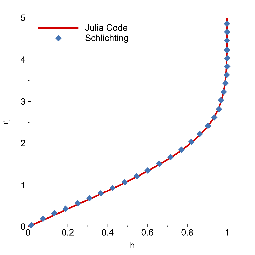
The solution vector is ploted and compared with results from Schlichting's Boundary-layer theory book.
Please read the full paper for further details.
Feel free to ask questions!
Furkan Oz
foz@okstate.edu
Kursat Kara
kursat.kara@okstate.edu
