This is an unpublished ongoing student project of vegetation response to meteorological drought using Google Earth Engine (GEE).
This is part of a group work about drought analysis by MSc students in Department of Earth Sciences, Uppsala University: de Mendonça Fileni, Felipe; Erikson, Torbjörn-Johannes; Feng, Shunan
Supervisor: Pettersson, Rickard; Winterdahl, Mattias
Preliminary results were presented during EGU general assembly 2019 in Vienna. EGU 2019-19137 Now we have expanded the study to global scale.
For questions regarding the script, please leave a comment or contact Shunan Feng.
SPEI is computed using the R package: Beguería S. (2017) SPEIbase: R code used in generating the SPEI global database, doi:10.5281/zenodo.834462. The 0.25 degree NOAH data is downloaded by from earthdata.nasa.gov by using EarthdataDownload.py. Note:
- NOAH data is in a different format as the input required by SPEIbase, the suggestion is to convert it to the same format as the data used in the SPEI template.
- GEE does not accept netcdf file, so we did an extra step to convert SPEI.nc to .tif.
- The link to the re-computed SPEI product will be available after the submission of the manuscript.
The global scale study utilizes MODIS 1km NDVI product. It explores the relationship between: 1) months of the sum of NDVI anomalies; 2) month lag of NDVI anomalies; 3) time scales of SPEI.
change the month lag here, e.g. no lag is 0, -1 is one month lag,-2 is 2 month lag. SPEI1-12m are available. Here we are only focusing on the drought so SPEI > 0 is masked. (by default, spei mask in uncommented)
var lagflag = 0;
var spei = spei11m.filterDate(date_start, date_end)
                  .map(function(image) {
                    var speiMask = image.lte(0);
                    return image.updateMask(speiMask);
                }); // mask out spei
Three layers will be displayed on the code editor interface:
- correlation map: Pearson correlation coefficient (R) of SPEI vs NDVI anomalies, pixels with p-value 0.05 will be masked.
- mean annual precipitation
- mean annual temperature
You can export the correlation map for further analysis by running the task.
This step correlates SPEI with NDVI anomalies in the selected month only. define the growth season (selected month of spei) here. e.g. the default setting is to correlate the SPEI in April in the study period with the NDVI anomalies.
var speim = 4;// month of spei This script utlizes Landsat data for time series analysis. It will import the shapefile produced from step 2.1. The vector layer covers areas where vegetation is sensitive to meteorological drought. Please draw or define your study area and rename it as roi before run this code.
 Three time series plots of monthly average NDVI, NDVI anomaly and SPEI will be displayed in the console.
2.4 SPEI Viewer
The purpose of the script is to provide a quick access to the SPEI product.computes the differences of the annual average SPEI. Positive SPEI values are masked as it focuses on the drought period. The difference maps show the annual difference of drought. Each layer represents the difference between the annual average SPEI in that year and its previous years.
Optionally, the export of the differences maps and the display of time series of SPEI at the defined study site

(stopped updating after April 2019)
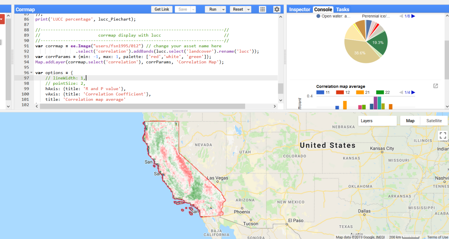
It exports and displays the correlation map of monthly SPEI vs the sum of coming three-month NDVI anomalies. The example in this script is studying California, 1984-2018. But it could also be applied to other areas by changing several lines of script.
Instruction:
- SPEI 2m Cal https://code.earthengine.google.com/?asset=users/felipef93/SPEI_CAL
- SPEI 3m Cal https://code.earthengine.google.com/?asset=users/felipef93/SPEI_CAL_3m
Change the study time here:
// study time range
var year_start = 1984;
var year_end = 2018;
// month range of ndvi anomalies (May to July)
var month_start = 5;
var month_end = 7;
var speim = 4;// month of spei
The example computes the three-month (May, June, July) sum of NDVI anomalies from 1984 to 2018 and correlates with SPEI in April.
For shorter period the correlation map could be displayed directly in GEE. For longer period, the results must be exported through tasks in GEE. The map could be exported to google drive or saved as GEE assets.
The correlation map exported to GEE asset from SEPI vs NDVI.js could be diaplayed and analyzed in this script. R and P values would be reported by different land cover. change your asset name here before run:
var corrmap = ee.Image("users/fsn1995/012") // change your asset name hereNDVI vs Water Balance NOAH.js Discarded personal practice withspatial correlation of water balance(NOAH 0.25 degree) and NDVI (landsat 30m)
- Vicente-Serrano S.M., Santiago Beguería, Juan I. López-Moreno, (2010) A Multi-scalar drought index sensitive to global warming: The Standardized Precipitation Evapotranspiration Index - SPEI. Journal of Climate 23: 1696-1718.
- Vicente-Serrano, S.M., Gouveia, C., Camarero, J.J., Begueria, S., Trigo, R., Lopez-Moreno, J.I., Azorin-Molina, C., Pasho, E., Lorenzo-Lacruz, J., Revuelto, J., Moran-Tejeda, E., Sanchez-Lorenzo, A., 2013. Response of vegetation to drought time-scales across global land biomes. Proceedings of the National Academy of Sciences 110, 52–57. https://doi.org/10.1073/pnas.1207068110
- Beguería, S., Vicente-Serrano, S.M., Fergus Reig, Borja Latorre. Standardized Precipitation Evapotranspiration Index (SPEI) revisited (2014): parameter fitting, evapotranspiration models, kernel weighting, tools, datasets and drought monitoring. International Journal of Climatology, 34: 3001-3023
- Sazib, N., Mladenova, I., Bolten, J., 2018. Leveraging the google earth engine for drought assessment using global soil moisture data. Remote Sensing 10. https://doi.org/10.3390/rs10081265
Fileni, F., Feng, S., Erikson., T, Winterdahl, M., Pettersson, R., 2019. Spatial and temporal analysis of vegetation response to meteorological droughts in California, 1984-2018