Behavioral Cloning Project
Design, train and validate a model for predicting steering angles from image data
The steps of the project are the following:
- Data acquisition with the Udacity simulator
- Data exploration
- Data augmentation
- Building of a convolutional neural network in Keras for predicting steering angles from images
- Model training and validation
- Test of the trained model with the Udacity simulator
- Video recording of the vehicle driving one full lap autonomously
The project includes the following files:
- model.py: containing the script to create and train the model
- drive.py: for driving the car in autonomous mode
- model.h5: containing the trained convolutional neural network
- README.md: summarizes the results
- video.mp4: recorded driving in autonomous mode
- data_exploration.ipynb: jupyter notebook for data exploration
- data_exploration.html: html file of the executed .ipynb file
Using the Udacity simulator and the drive.py file, the car can be driven autonomously around the trach by executing
python drive.py model.h5Since the NVIDIA model from the End to End Learning for Self-Driving Cars paper was designed exactly for this purpose, I adapted the model for this project.
The model is basically a convolutional neural network (CNN) with five convolutional layers and three fully connected layers and is shown below.
- Normalization and Downsampling: After normalizing the input images in the first layer, the images are downsampled by 2 in the second layer to reduce training time.
- Gaussian noise: The next layer adds gaussian noise to the images to avoid using identical flipped images for training. The layer has a regularizing effect and is only active during training.
- Convolutional layers: Next, five convolutional layers are added. Like the NVIDIA model, the first three layers use a 5x5 Kernel with 2x2 stride followed by two layers with 3x3 Kernel and 1x1 stride.
- Flatten and Dense layers: After flattening the 2D images, the model consists of three fully connected layers with a dropout layer for each to avoid overfitting.
Since it is a regression network which is supposed to output a continuous steering angle, the last layer consists of a single node without an activation function. For minimizing the error between the predicted steering angles and the ground truth steering angles, mean squared error (mse) is used as loss function.
Model: "sequential_2"
_________________________________________________________________
Layer (type)                 Output Shape              Param #
=================================================================
lambda_2 (Lambda)            (None, 160, 320, 3)       0
_________________________________________________________________
max_pooling2d_2 (MaxPooling2 (None, 80, 160, 3)        0
_________________________________________________________________
gaussian_noise_2 (GaussianNo (None, 80, 160, 3)        0
_________________________________________________________________
conv2d_6 (Conv2D)            (None, 38, 78, 24)        1824
_________________________________________________________________
conv2d_7 (Conv2D)            (None, 17, 37, 36)        21636
_________________________________________________________________
conv2d_8 (Conv2D)            (None, 7, 17, 48)         43248
_________________________________________________________________
conv2d_9 (Conv2D)            (None, 5, 15, 64)         27712
_________________________________________________________________
conv2d_10 (Conv2D)           (None, 3, 13, 64)         36928
_________________________________________________________________
flatten_2 (Flatten)          (None, 2496)              0
_________________________________________________________________
dense_5 (Dense)              (None, 100)               249700
_________________________________________________________________
dropout_4 (Dropout)          (None, 100)               0
_________________________________________________________________
dense_6 (Dense)              (None, 50)                5050
_________________________________________________________________
dropout_5 (Dropout)          (None, 50)                0
_________________________________________________________________
dense_7 (Dense)              (None, 10)                510
_________________________________________________________________
dropout_6 (Dropout)          (None, 10)                0
_________________________________________________________________
dense_8 (Dense)              (None, 1)                 11
=================================================================
Total params: 386,619
Trainable params: 386,619
Non-trainable params: 0
_________________________________________________________________
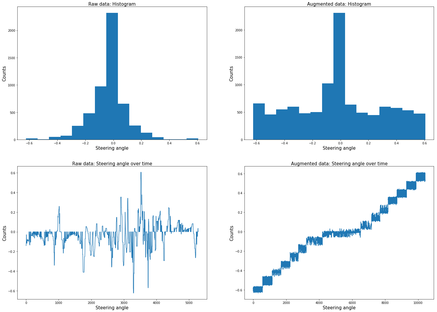
The dataset basically consists of one round of driving in the middle of the road as precisely as possible and one recovery round, where the recording was started at the side of the road and steered back to the center. Additionally, the two curves with high curvature were driven again. The raw dataset consists of 5283 images.
Since the data is highly unbalanced with most samples at zero angle, those samples with angles unequal zero were duplicated. The resulting distribution is shown below. The augmented data has length 10431.
In addition, the images of all three cameras are used with an offset angle of 0.2 for the left image and -0.2 for the right image. Since training data is biased towards the left, a flipped version of each image is included to the dataset, too.
Eventually, the full augmented data set consists of 62586 samples.
To avoid using the identical duplicated images for training, a noise layer was added to the network.
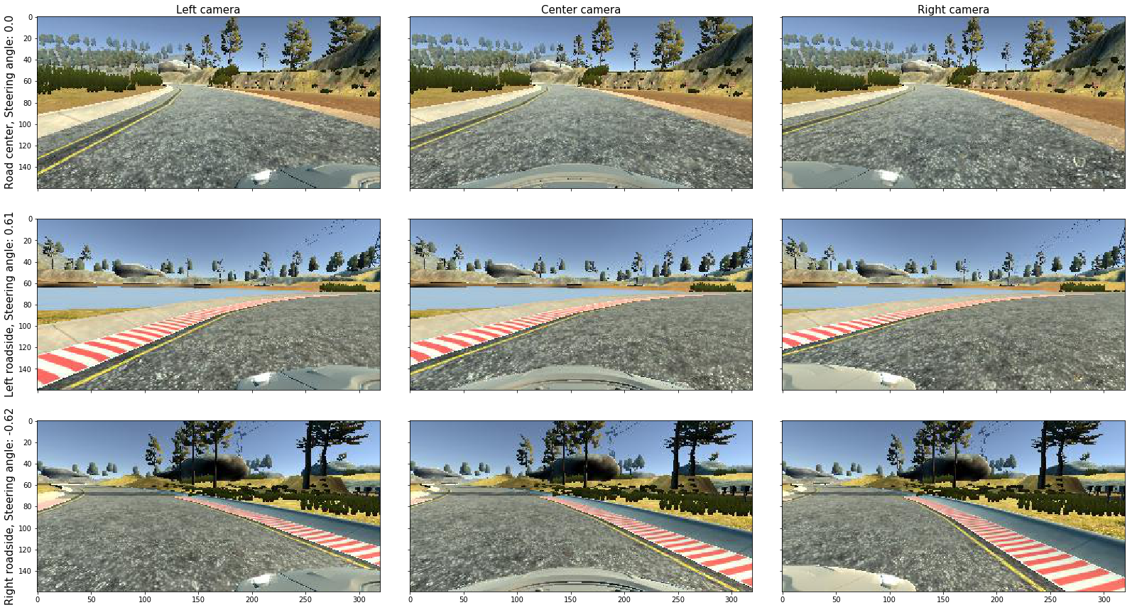
Example images are provided below for different steering angles and all three camera positions.

Following plots show the steering angle distribution and angle over time of the raw data set on the left and the augmented data set on the right. Since the car drove zig-zag with uniform steering angle distribution, the distribution in the upper right was chosen.

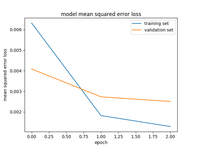
A generator was used for loading the images in batches instead of all at once. Training was done using ADAM optimizer which includes an adaptive learning rate. The model was trained for 5 epochs with a batch size of 32. The recorded data was split into a training set of 80% of the images and a validation set of 20%. For regularization, a gaussian noise layers and dropout layers were used. The following figure shows the mean squared error loss for the 3 epochs. The model tends to overfit, but since the error is relatively small and the model shows an acceptable driving behavior, regularization was not further increased.
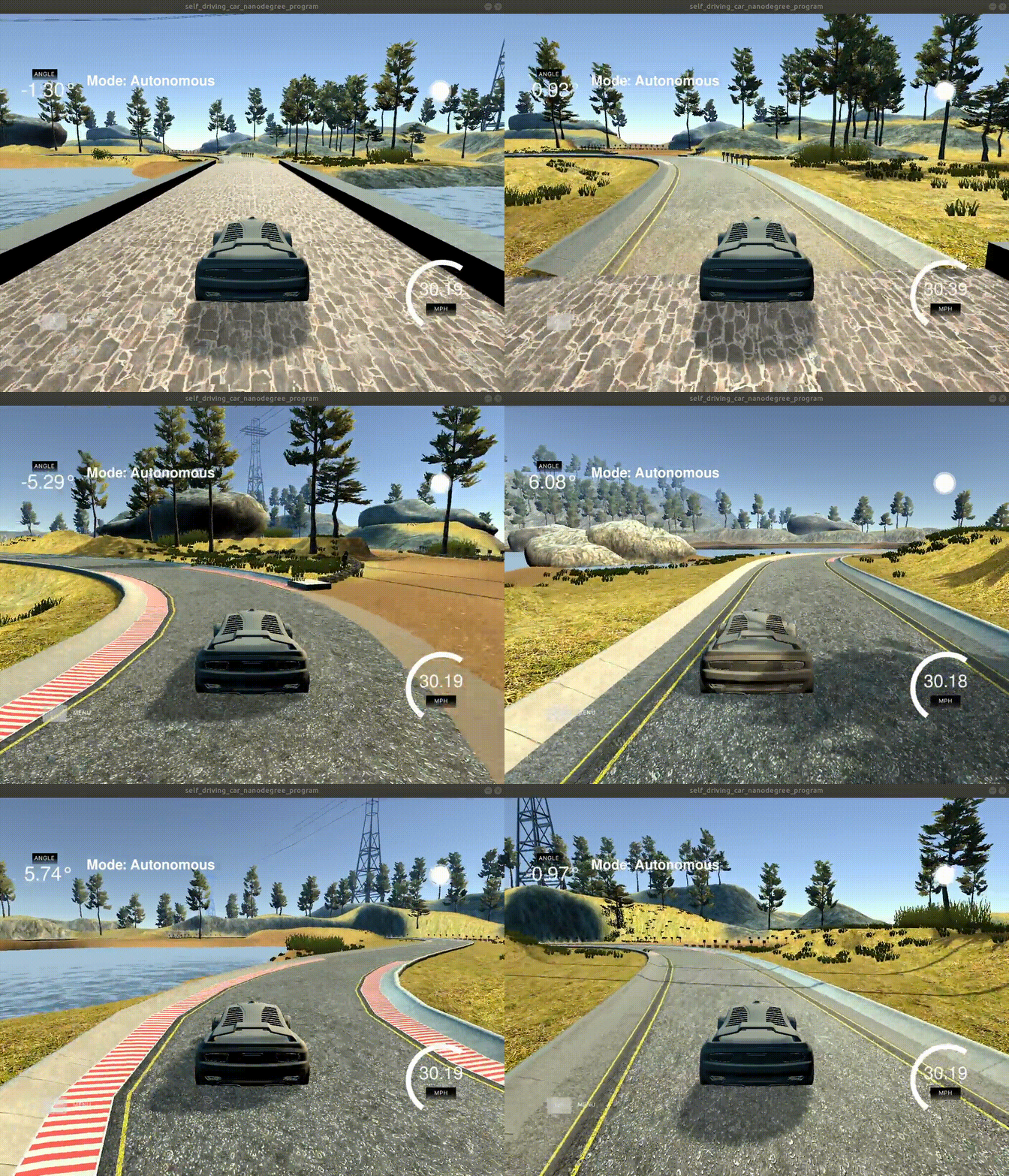
The vehicle was driven at 30 mph autonomously on the whole track, which can be seen in the included video.mp4 file. The following gif shows the vehicle driving the two hardest curves of the track.


