Implementation of particle swarm optimization (PSO) for path planning when the environment is known.
-
The code has been written and tested in Python 3.8.5.
-
Four types of obstacles: circle, ellipse, convex polygon, generic polygon.
-
Start position, goal position, and obstacles can be dynamically changed to simulate motion.
-
Penalty function of type
1/xwith the center in the obstacle centroid*. -
To improve the execution speed, the algorithms to determine if a point is inside an obstacle have been designed to carry out the determination on all points simultaneously.
-
Points on the obstacle borders/edges are not considered inside the obstacle.
-
Option to run sequential tests with different initial conditions to increase the chances to find a global minimum.
-
Usage: python test.py example.
*Some centroid may be outside the obstacle, such as the U-shaped element in the below examples. If that is a problem the simples solution is to divide the obstacle in smaller shapes using convex polygons. For instance, for the mentioned U-shape obstacle two vertical and one horizontal polygons could be used.
example Number of the example to run (1, 2, or 3.)
start Start coordinates.
goal Goal coordinates.
limits Lower and upper boundaries of the map and search space in the PSO.
nRun Number of runs.
nPts Number of internal points defining the spline. The number of variables is twice this number.
d Number of segments between the spline breakpoints.
nPop, epochs Number of agents (population) and number of iterations.
f_interp Order of the spline (1st, 2nd and 3rd order, respectively.)
Xinit Initial value of the variables. Set Xinit=None to pick them randomly. This array is organized with first the x-coordinates of all internal points and then the y-coordinates of all internal points.
K Average size of each agent's group of informants. If K=0 the entire swarm is used as agent's group of informants.
phi Coefficient to calculate the self-confidence coefficient and the confidence-in-others coefficient.
vel_fact Velocity factor to calculate the maximum and the minimum allowed velocities.
conf_type Confinement type (on the velocities): HY=hyperbolic, RB=random-back, MX=mixed hyeperbolic/random-back.
IntVar List of indexes specifying which variable should be treated as integer. If all variables are real set IntVar=None, if all variables are integer set IntVar=all.
normalize Specifies if the search space should be normalized (to improve convergency).
rad Normalized radius of the hypersphere centered on the best particle. The higher the number of other particles inside and the better is the solution.
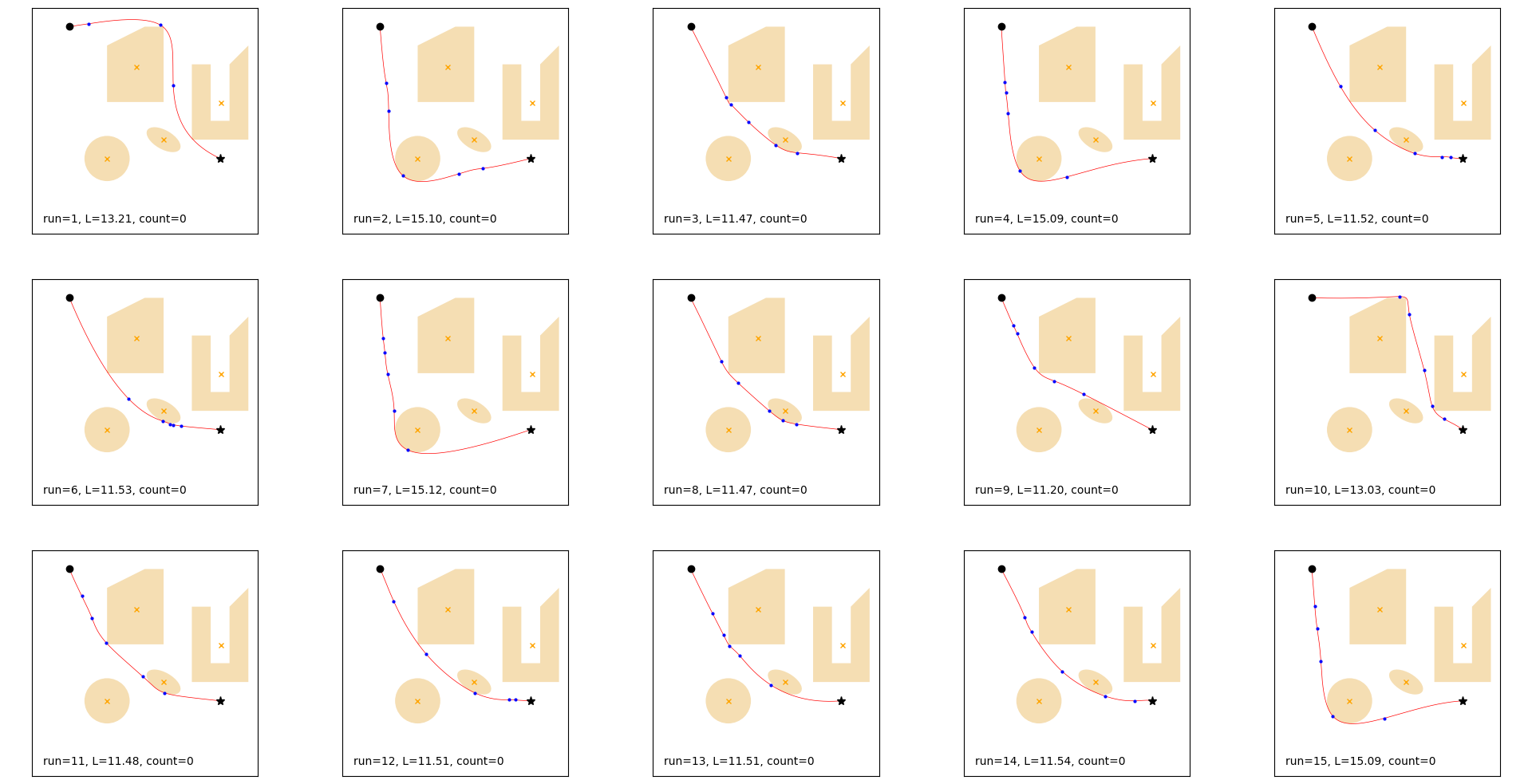
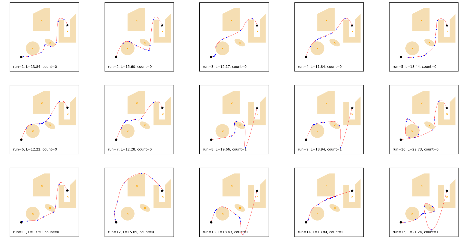
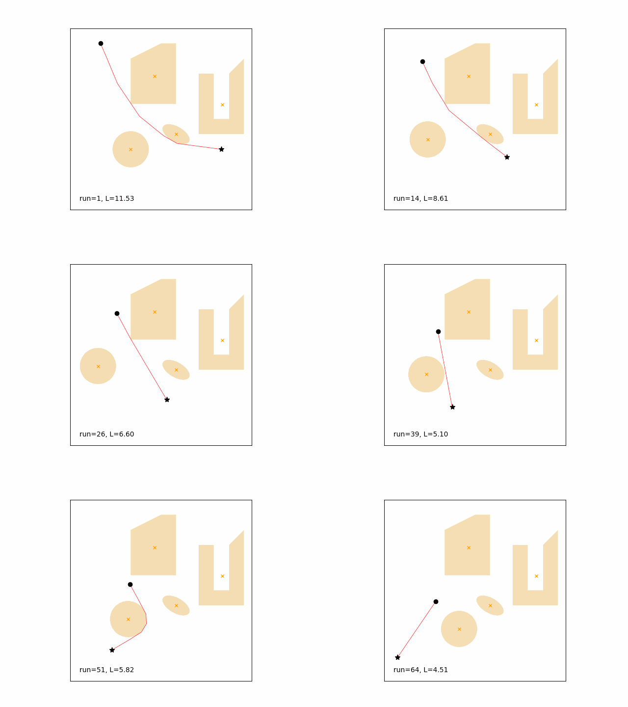
There are three examples, all of them using the same obstacles:
Example 1
-
Multiple runs, cubic spline, optimizer initialized randomly.
-
Best: run=9, L=11.20, count=0.
-
No obstacle violations.
-
See the code for the parameters used.
Example 2
-
Multiple runs, quadratic spline, optimizer initialized with the straight line between start and goal position.
-
Best: run=4, L=11.884, count=0.
-
Obstacle violation in run 8, 9, 13, 14, and 15.
-
See the code for the parameters used.
Example 3
-
Single run, linear spline, optimizer initialized with the previous solution, start point chasing a moving goal with one obstacle (the circle) also moving.
-
Path length goes from 11.53 (run 1) to 4.52 (run 65).
-
No obstacle violations.
-
See the code for the parameters used.


