Solar segmentation

Finding solar panels using USGS satellite imagery.

1. Introduction

This repository leverages the distributed solar photovoltaic array location and extent dataset for remote sensing object identification to train a segmentation model which identifies the locations of solar panels from satellite imagery.

Training happens in two steps:

Using an Imagenet-pretrained ResNet34 model, a classifier is trained to identify whether or not solar panels are present in a [224, 224] image.
The classifier base is then used as the downsampling base for a U-Net, which segments the images to isolate solar panels.

2. Results

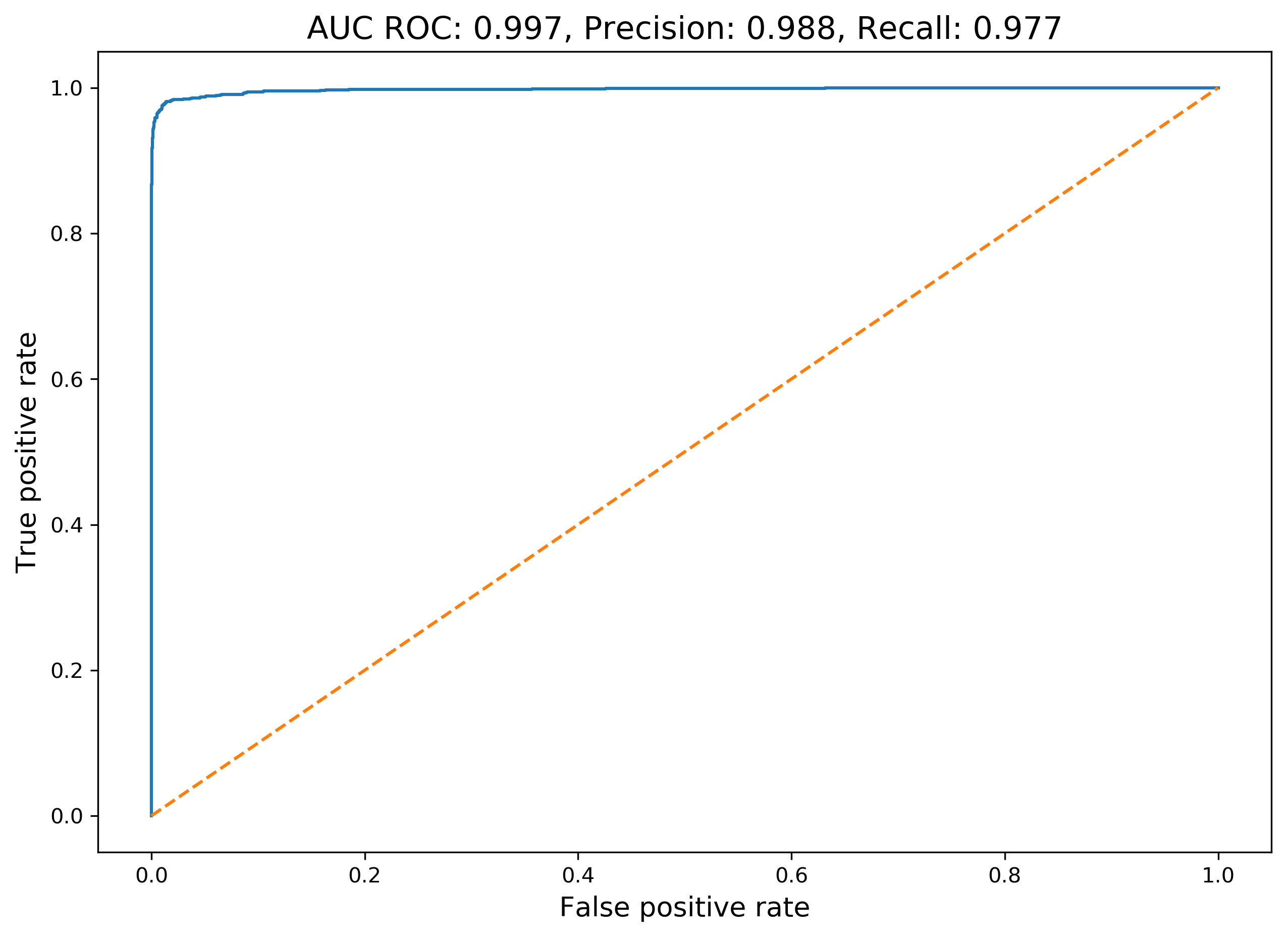
The classifier was trained on 80% of the data, with 10% being used for validation and 10% being used as a holdout test set. On this test set, with a threshold of 0.5 differentiating positive and negative examples, the model achieved a precision of 98.8%, and a recall of 97.7%. This is competitive with DeepSolar (precision of 93.1% - 93.7%, and recall of 88.5% - 90.5%) despite being trained on a smaller, publically available dataset.

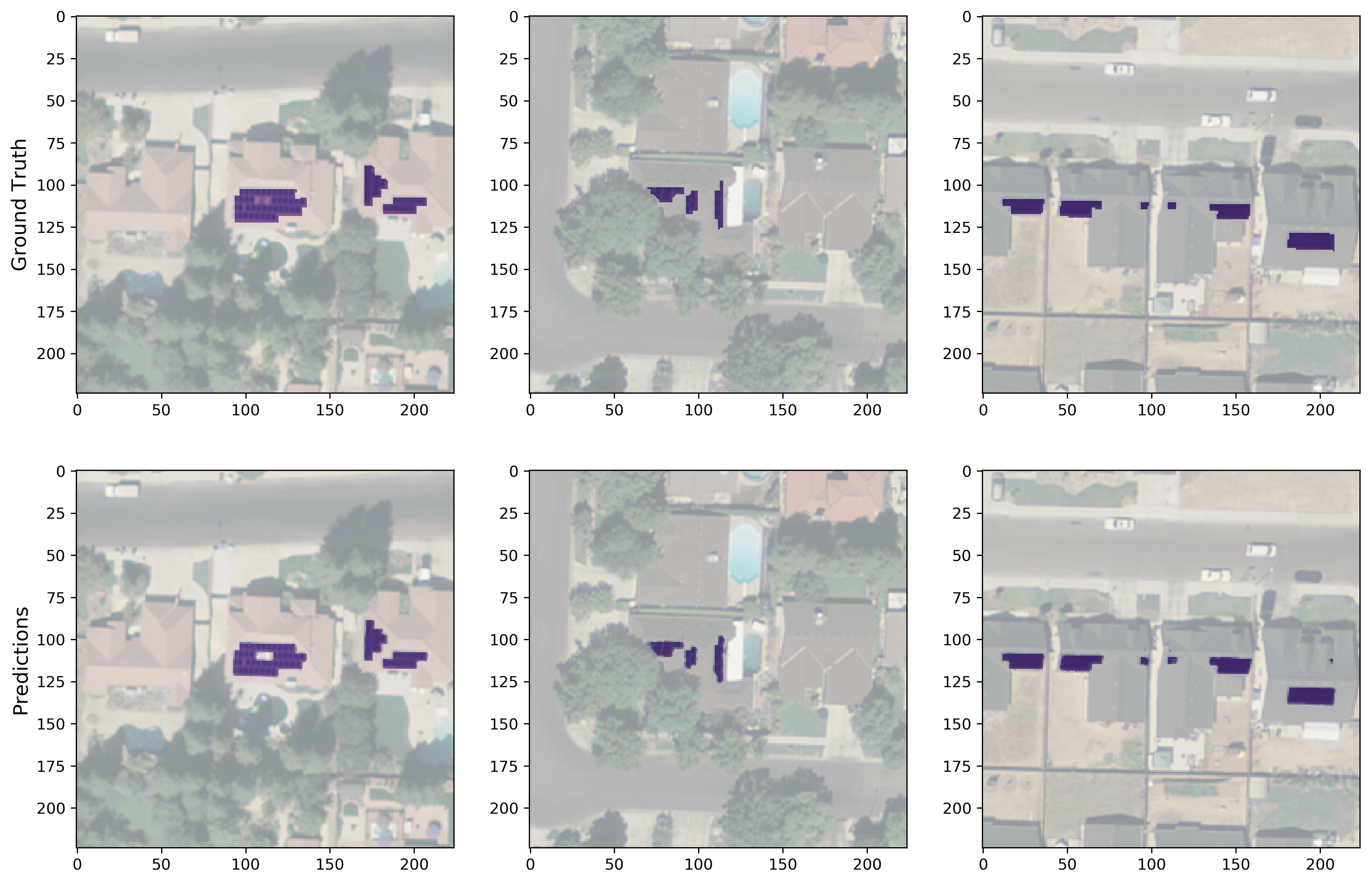
The segmentation model achieved a Dice coefficient of 0.89:

3. Pipeline

The main entrypoint into the pipeline is run.py. Note that each component reads files from the previous step, and saves all files that later steps will need, into the data folder.

In order to run this pipeline, follow the instructions in the data readme to download the data.

Python Fire is used to generate command line interfaces.

3.1. Make masks

This step goes through all the polygons defined in metadata/polygonVertices_PixelCoordinates.csv, and constructs masks for each image, where 0 indicates background and 1 indicates the presence of a solar panel.

python run.py make_masks

This step takes quite a bit of time to run. Using an AWS t2.2xlarge instance took the following times for each city:

Fresno: 14:32:09
Modesto: 41:48
Oxnard: 1:59:20
Stockton: 3:16:08

3.2. Split images

This step breaks the [5000, 5000] images into [224, 224] images. To do this, polygonDataExceptVertices.csv is used to identify the centres of solar panels. This ensures the model will see whole solar panels during the segmentation step.

Negative examples are taken by randomly sampling the image, and ensuring no solar panels are present in the randomly sampled example.

python run.py split_images

This yields the following images (examples with panels above, and without below):

3.3. Train classifier

This step trains and saves the classifier. In addition, the test set results are stored for future analysis.

python run.py train_classifier

3.4. Train segmentation model

This step trains and saved the segmentation model. In addition, the test set results are stored for future analysis. By default, this step expects the classifier to have been run, and will try to use it as a pretrained base.

python run.py train_segmenter

Both models can be trained consecutively, with the classifier automatically being used as the base of the segmentation model, by running

python run.py train_both

4. Setup

Anaconda running python 3.7 is used as the package manager. To get set up with an environment, install Anaconda from the link above, and (from this directory) run

conda env create -f environment.{mac, ubuntu.cpu}.yml

This will create an environment named solar with all the necessary packages to run the code. To activate this environment, run

conda activate solar

This pipeline can be tested by running pytest.

Docker can also be used to run this code. To do this, first build the docker image:

docker build -t solar .

Then, use it to run a container, mounting the data folder to the container:

docker run -it \
--mount type=bind,source=<PATH_TO_DATA>,target=/solar/data \
solar /bin/bash

gabrieltseng/solar-panel-segmentation