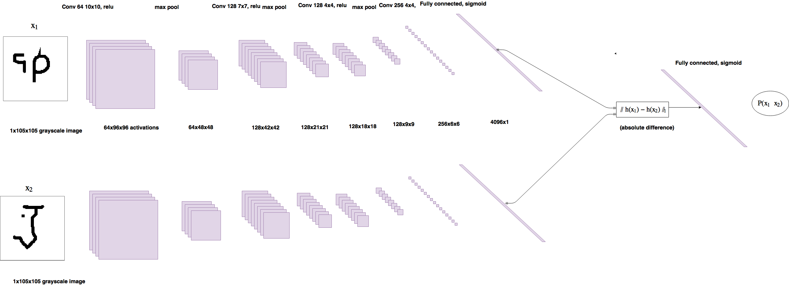
Typical CNN classification methods involve a final fully-connected layer with neurons corresponding to the number of classes. This is suboptimal in situations where the number of classes is large, or changing.
In Siamese CNNs, we extract features from an image and convert it into an n-dimensional vector. We compare this n-dimensional vector with that of another image, and the model is trained such that images of the same class will produce similar vectors.
By comparing an unknown image against samples of labelled images, we are able to determine the labelled image which is most similar to the unknown image, and obtain a classification result. This provides Siamese networks with the ability to learn classification tasks with low training samples, as well as generalize to any number of classes.
Much like a typical CNN, a Siamese CNN will have several convolutional layers, followed by fully-connected layers. The convolutional layers help to extract features from an image, before conversion into vectors for comparison.
When training a Siamese CNN, we input two images, and a binary label indicating if the two images are of the same class. The last layer of the CNN is a fully-connected layer, which produces an n-dimensional vector. Subsequently, the output layer and the output vector will be used interchangably, and both refer to this layer. Depending on the label, the model will then try to minimize or maximize the distance between the vectors produced by the two images.
Note that the network that both images pass through are the same. This means that the weights and biases in the network for both images are identical throughout the training process.
In this project we experiment with two different kinds of loss functions. The loss is calculated based on the L1- or L2-distance between the outputs of the CNN (fully-connected layers) from the two images.
In Dimensionality Reduction by Learning an Invariant Mapping the loss function as shown below is described. The following GitHub project is used as reference for the implementation of the loss function.
Sigmoid loss for image recognition in Omniglot dataset is used in the paper Siamese Neural Networks for One-shot Image Recognition. The model architecture used in the paper is also the basis for the CNN for the Omniglot task.
We start with MNIST to test our implementation. The model was trained with learning_rate=1e-4 over 20,000 iterations. The training results for several architectures are summarized below:
| commit_hash | conv. kernel size | accuracy | description |
|---|---|---|---|
983a8a8 |
3x3 |
0.9758 | 2 layer FC + 2-neuron out |
df5d2b9 |
5x5 |
0.9844 | 2 layer conv + 2 layer FC + 2-neuron out |
df5d2b9 |
3x3 |
0.9856 | 2 layer conv + 2 layer FC + 2-neuron out |
3757780 |
3x3 |
0.9890 | 2 layer conv + 2 layer FC (out) |
We first train a CNN on an MNIST classification task, achieving 99.37% accuracy on the test set. We then transfer the weights from the convolutional layers to the Siamese CNN before training the Siamese model with learning_rate=1e-4 over 10,000 iterations. This achieved a test accuracy of 98.99%, higher than the current maximum attained without transfer learning.
For each of the ground truth images above, we obtain its output vector via the model. Then, for each image that we are evaluating, we obtain its output vector as well, then find the closest ground truth vector to it via L1- or L2-dist.
The Omniglot dataset is typically used for one-shot learning, as it contains a large number of classes, with few training samples per class.
While the training and testing classes were the same in MNIST, the Omniglot dataset allows us to test the model on completely different classes from the ones used in training.
A random seed of 0 was set for both the Python inbuilt random library, as well as Tensorflow.
Images in the images_background folder were used for training. For each class (e.g. Alphabet_of_the_Magi/character01), all possible combinations of pairs were appended to a list. For example, a class with 20 images yielded 20 choose 2 == 190 pairs.
n_samples number of pairs were then chosen at random from the possible pairs to form the training data for similar images. Subsequently, for each similar pair, we add a dissimilar pair by choosing two different classes at random, and choosing one image each from both classes. This ensures that the number of similar and dissimilar pairs are the same.
Images in the images_evaluation folder were used for testing. We use 20 classes (Angelic/character{01-20}) for testing, and determine accuracy by the number of correct predictions.
| model_name | n_samples | n_iterations | learning_rate | dist | accuracy |
|---|---|---|---|---|---|
fc1 |
20 000 | 50 000 | 1e-5 | L1 | 0.4025 |
fc1 |
20 000 | 50 000 | 1e-5 | L2 | 0.4150 |
fc1 |
40 000 | 50 000 | 1e-5 | L1 | 0.4000 |
fc1 |
40 000 | 50 000 | 1e-5 | L2 | 0.4000 |
fc1_reg1 |
20 000 | 50 000 | 1e-5 | L1 | 0.2700 |
fc1_reg1 |
20 000 | 50 000 | 1e-5 | L2 | 0.2725 |
fc2 |
20 000 | 50 000 | 1e-5 | L1 | 0.2875 |
fc2 |
20 000 | 50 000 | 1e-5 | L2 | 0.2800 |
Single fully-connected layer with 4096 neurons.
Regularization with 2e-4 for convolutional layers.
Two fully-connected layer with 2048 neurons each, dropout=0.5 between fc1 and fc2. Number of neurons was reduced due to OOM allocations.


