Segmenting the Iowa Wholesale Liquor Market

The Data Incubator
2020 Fall
Capstone Project

1 Business Objective

This product uses machine learning (feature engineering and density-based clustering) to partition the Iowa liquor market into discrete components. Market segmentation will benefit wholesalers (the intended user) by allowing them to:

target advertising by region
identify potential buyers (liquor stores)
more effectively partition sales regions for salespersons

In Iowa, wholesale liquor is a 300 million dollar a year market (see Table 1) with 452 sellers (brands/manufacturers) and 2415 buyers (liquor stores) (see Note 2). Wholesale transactions are reported to the Iowa Alcoholic Beverages Division, who make the data (from 2012 to present) available at: https://data.iowa.gov/Sales-Distribution/Iowa-Liquor-Sales/m3tr-qhgy The dataset consists of about 19 million transactions from 2012 through the present, and is about 4.5 GB [See Table 3 below].

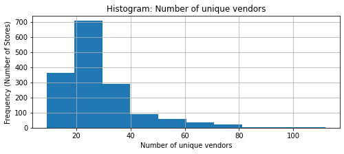
Each liquor store typically carries around 35 brands (see Table 4 below), and each brand employs salespersons that work the a number of liquor stores. For context, in the Manhattan liquor market, a salesperson might have a territory of 50 liquor stores.

Table 1

	Brandy	Cocktail	Gin	Liqueur	Neutral	Rum	Tequila	Vodka	Whiskey	All
USD (Millions)	14.58	4.37	7.27	44.82	0.85	32.95	19.77	73.73	99.17	297.50
Liters (Millions)	0.60	0.60	0.49	2.65	0.04	2.34	0.85	6.28	5.19	19.05
Gallons (Millions)	0.16	0.16	0.13	0.70	0.01	0.62	0.22	1.66	1.37	5.02

Note 2

Note that the Iowa wholesale market excludes on-premise retailers (ie, restaurants and bars), who must buy through an off-premise retailer (ie, a liquor store).

Table 3

	filename	filesize	number of rows
Raw data	raw.csv	4.5G	19 884 006
Cleaned data	data.parquet	848M	19 883 991
nonanomalous rows only			18 409 105
Downsampled data (5%)	downsample.parquet	47M	993 222

Table 4

See 4-feature-engineering.ipynb

	%Vodka	%Whiskey	%Neutral	#Cat	#Invoice	#Item	#Vendor_num	Total$	Latitude	Longitude	$/gal_tequila	$/gal_all
mean	0.26	0.33	0.0019	8	1230	232	28	187595	41.9753	-93.0522	109	58

2 Data Ingestion

See 2-data-ingestion.ipynb

The dataset after cleaning and formatting (but before feature engineering) has 25 columns. See Table 5 for summary stats for 12 columns. By cleaning the data we are able to reduce the filesize from 4.5 GB to 848 MB. (See Table 3 above.)

After removing some anomolies, the Invoice column becomes a uniquely identifying column, so we could write df = df.set_index('Invoice'). However, we keep the index as is in case users run these notebooks in future months without manually cleaning any new anomolies the have appeared in the Iowa Alcoholic Beverages Division dataset.

After cleaning, we add the new feature Category, which groups of the subcategories in the original dataset into 9 major categories. We also use detect errors in the data by investigating outliers (such as locations not in Iowa) and by comparing redundant features (such as checking Bottle_cost times Bottle_count equals Cents).

Finally we generate a random column and use it to take a 5% sample to assist in later analysis.

Table 5

	dtype	count	null count	unique	top	freq	first	last
Date	datetime64[ns]	19883991	0	2157	2017-12-22	16674	2012-01-03	2020-10-30
Invoice	object	19883991	0	19883991	128404200011	1
Store	object	19883991	0	2613	Hy-Vee #3 / Bdi / Des Moines	169816
Address	object	19804064	79927	2415	3221 Se 14Th St	231054
City	object	19804065	79926	456	Des Moines	1730907
Subcategory	object	19858951	25040	110	Canadian Whiskies	1916720
Vendor	object	19883991	0	452	Diageo Americas	3356016
Item	object	19883991	0	8666	Black Velvet	515736

	dtype	count	null count	mean	std	min	0.01%	99.99%	max
Cents	int32	19883991	0	13527	47022	0	0	1620000	27955728
Gallons	float32	19883991	0	2	9	0	0	277	3963
Longitude	float32	17976922	1907069	-91	3	-105	-97	-90	-74
Latitude	float32	17976922	1907069	42	1	39	40	43	45

3 Visualization

Choropleth

See 3-choropleth.ipynb

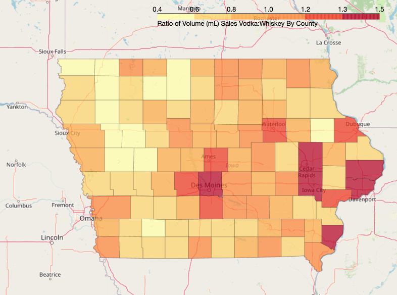
The Iowa liquor market is not homogeneous. For example, consider the ratio of sales of vodka to sales of whiskey. Regions around Des Moines, Davenport, Cedar Rapids, and Iowa City purchase more vodka then whiskey, perhaps due to restaurant density. The rest of Iowa purchases more whiskey than vodka.

Time Series

See 3-time-series.ipynb

The market has been growing since 2012. However, growth is mostly driven by vodka and whiskey, and more recently, Liqueur.

Looking at sales of all categories and overlaying years 2012-2020, we see that this secular growth trend in the market is not limited to any particular time of year.

Averaging over all years, liquor purchases are highest in October, November, December. However, this cyclical increase is entirely driven by whiskey in Iowa. In the NYC liquor market, sales of both whiskey and vodka go up in the 4th quarter, as restaurants serve more vodka-based mixed-drinks. In future analysis, cyclical changes in vodka purchases (aggregated by liquor store) may allow us to identify which liquor stores sell extensively to restaurants, and which liquor stores mostly sell directly to consumers.

We can also aggregate by Item. Since the same product may be sold over different names, we need to group the items by keyword into product lines. TF-IDF can be used to find keywords that are rare overall, but common for a single brand, however the keywords generated were not as good a brand-exclusivity search. See 3-time-series.ipynb. In future analyses, TF-IDF cosine similarity may allow us to cluster items into product lines directly.

We see that sales have not improved for every product line. For example, compare Tito's Vodka and Ciroc.

Note that Ciroc is a rapper-sponsored liqueur, and it is common knowledge in liquor sales that liqueurs tend to be more prone to fads.

4 Machine Learning

Feature Engineering

See 4-feature-engineering.ipynb

The original dataset, after cleaning, is a ledger of some 19 million transactions.

Here are the first 3 rows.

	Invoice	Date	Store_num	Store	Address	City	Zip	County_num	County	Subcategory_num	Subcategory	Vendor_num	Vendor	Item_num	Item	Bottle_pack	Bottle_mL	Bottle_cost	Bottle_retail	Bottle_count	Cents	mL	Gallons	Longitude	Latitude	Category	Anomalous	Random
0	126831400106	2020-04-27 00:00:00	2190	Central City Liquor, Inc.	1460 2Nd Ave	Des Moines	50314	77	Polk	1012100	Canadian Whiskies	260	Diageo Americas	10804	Crown Royal Regal Apple	44	200	472	708	6	4248	1200	0.31	-93.6198	41.6057	Whiskey	False	0.929616
1	126855200028	2020-04-27 00:00:00	5339	Prime Star	395 Western Avenue	Marengo	52301	48	Iowa	1901200	Special Order Items	330	Gemini Spirits	988037	Sooh Margaritaville Silver Tequila	12	1000	784	1176	2	2352	2000	0.52	-92.0744	41.793		False	0.316376
2	126788200025	2020-04-24 00:00:00	4092	Fareway Stores #077 / Norwalk	1711 Sunset Dr	Norwalk	50211	91	Warren	1031200	American Flavored Vodka	260	Diageo Americas	77994	Smirnoff Red, White & Berry	6	1750	1475	2213	30	66390	52500	13.86	-93.6755	41.4833	Vodka	False	0.183919

Before running cluster analysis on liquor store, we need to engineer a few features. To head of survivorship bias, we first filter to 2019 by writing df[df.Date.dt.year==2019]. Next we pivot the dataset by Store_num, meaning that the index will be Store_num Then we engineer the following features.

We aggregate by sum over Cents (sales) to get Totals sales.
We aggregate by nunique over Vendor_num, Category, Item_num, and Invoice to get the number of unique brands, unique categories (out of 9), unique items, as well as the total number of transactions.
We separately engineer the average price in dollars/gallon, still indexed by Store_num but now additionally columned by Category. In fact, we do this pivot and aggregate Gallons by sum, and then repeat with Cents (sales) to get (#1). We divide the two resulting dataframes to get dollars/gallon for each store, grouped by Category (there are 9).
Finally, we separately engineer the sales (USD) proportion by category by taking the previously defined dataframe (#1) and the dividing by its last column (All). Originally we also computed sales (gal)proportion by category, but dropped the feature as it is already adequately described by combine interaction of "sales (USD) proportion by category" and "dollars/gallon"

Feature selection

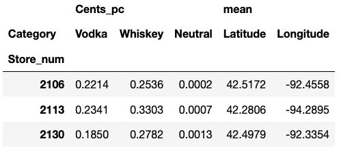
Finally I chose the following 12 features to run clustering on based on which ones had the largest standard deviation.

Here are the first 3 columns of the result.

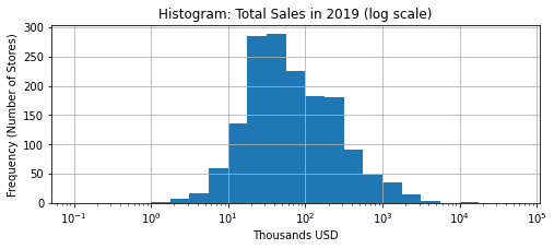
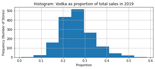
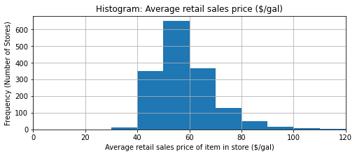
To better understand these new features, here are selected histograms. Observe that total sales is approximately exponentially distributed, whereas the others are approximately normal (with right-skew).

Clustering

See 4-clustering.ipynb

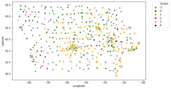
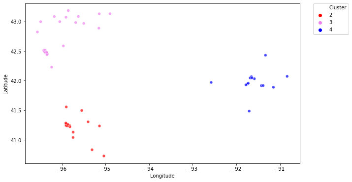
Using a density-based clustering algorithm on the features selected above produces 5 clusters, two that conver the whole state, and three localized clusters.

Interpretation

See tables at bottom of 4-clustering.ipynb

Cluster 0: everywhere in Iowa, portfolio of 30 vendors on average, 180k sales, carries 250 products, carries cheap tequila
Clusters 1-4: portfolio of 20 vendors, carries 100 products, carries expensive tequila and no/few neutral grain spirits
- Cluster 1 stores are everywhere in Iowa except the northwest, 50k in sales
- Cluster 2 stores carry less Vodka and less Whiskey than average, 60k in sales
- Cluster 3 stores are in the northwest and carry less Vodka and more Whiskey than average, 50k in sales
- Cluster 4 stores are in the eastern collegiate region of Iowaand sells more Vodka than Whiskey, 25k in sales; all carry exactly 0 neutral grain spirits,

This density-based clustering algorithm has difficulty classifying large liquor stores (average sales 350k, 35 brands) with expensive tequila. These may be due to larger warehouse-type stores being located in (relatively) geographically isolated lots with parking.

5 Deliverable

The current README

gatewaycat/iowa-liquor-sales2