Advanced Lane Finding Project
The goals / steps of this project are the following:
- Compute the camera calibration matrix and distortion coefficients given a set of chessboard images.
- Apply a distortion correction to raw images.
- Use color transforms, gradients, etc., to create a thresholded binary image.
- Apply a perspective transform to rectify binary image ("birds-eye view").
- Detect lane pixels and fit to find the lane boundary.
- Determine the curvature of the lane and vehicle position with respect to center.
- Warp the detected lane boundaries back onto the original image.
- Output visual display of the lane boundaries and numerical estimation of lane curvature and vehicle position.
1. Briefly state how you computed the camera matrix and distortion coefficients. Provide an example of a distortion corrected calibration image.
The code for this step and all other steps is contained in 'adv_lane_lines.py' file.
The objpoints and img point arrays are initiated as empty arrays. The calibration image file is read using cv2.imread function.
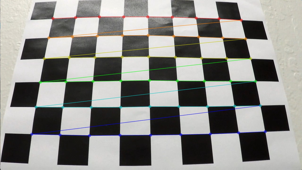
The cv2.cvtColor(img,cv2.COLOR_BGR2GRAY) function converts a 3 channel colored image to a grayscale image. cv2.findChessboardCorners(gray, (nx, ny), None) function with correct gird parameters (in this case 6x9 corners) results into detected corners stored in an array which is then appended to imgpoints. The object points is prepared using np.mgrid[0:9,0:6].T.reshape(-1,2) which is further appended to objpoints.
The object point and image point matrices are then used to perform calibration on the camera using the function cv2.calibrateCamera(objpoints, imgpoints, gray.shape[::-1], None, None). The cv2.calibrateCamera function returns distortion coefficients (dist), camera matrix (mtx), rotation and translation vectors (rvecs and tvecs).
The distortion coefficients along with camera matrix is used to undistort an image
undist = cv2.undistort(img, mtx, dist, None, mtx)
This returns an image (undist) which is free of any kind of distortion.
The camera is calibrated only once, the calibration coefficients are then stored in a pickle file named calibration_pickle.p
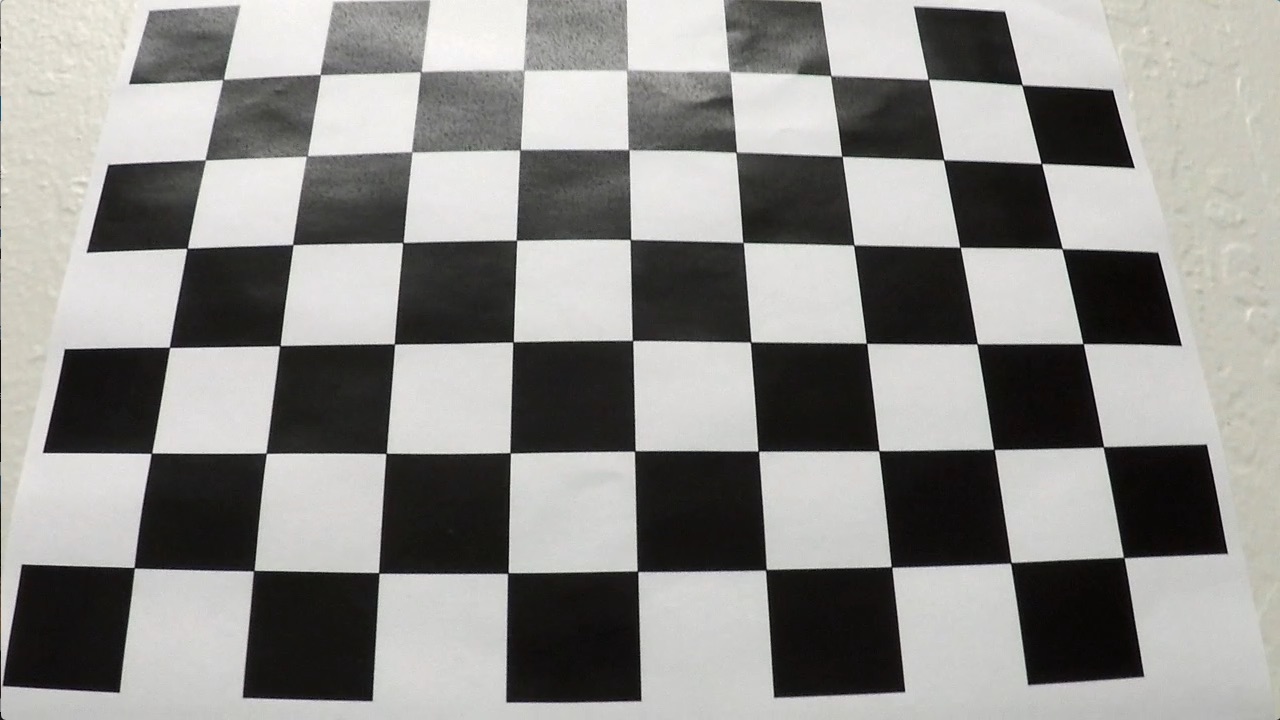
| Raw Calibration Image | Detected Corners | Undistorted Image |
|---|---|---|
 |
 |
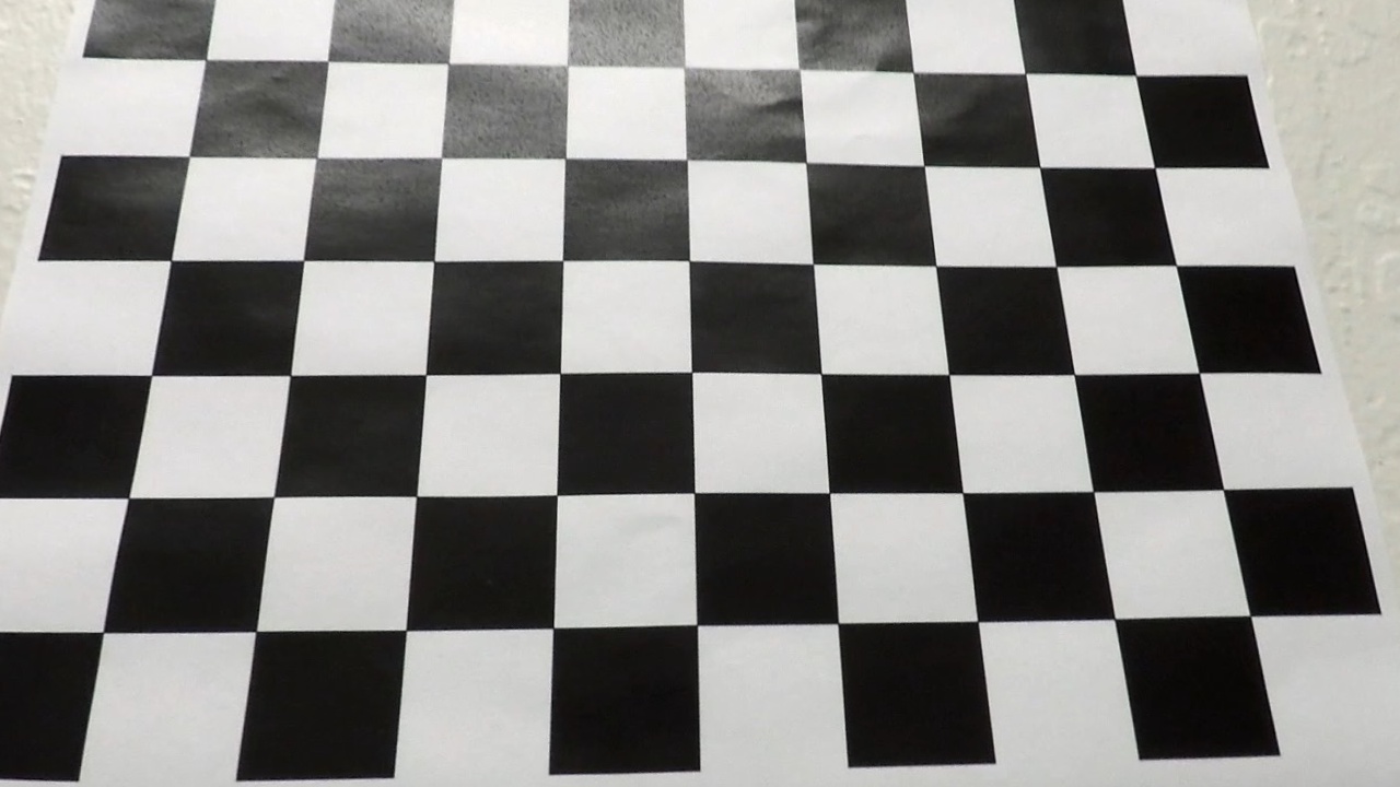 |
Figures show the raw calibration image, calibration image with detected corners and the image after applying distortion correction
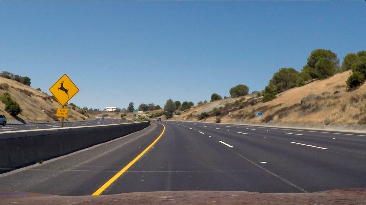
The cv2.undistort function is incorporated in the pipeline, so that distortion correction is applied to each image.
| Raw Camera Image | Undistorted Image |
|---|---|
 |
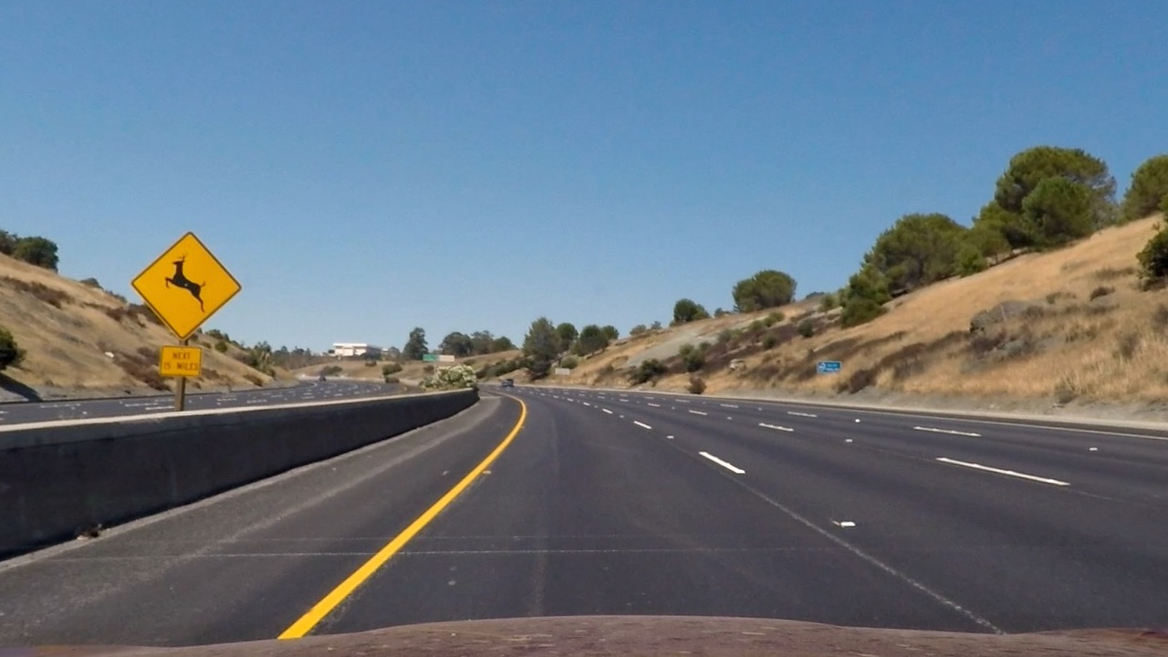 |
Figures show the raw camera image and the image after applying distortion correction. The car on the corner of the raw image is not visible in undistorted image
2. Describe how (and identify where in your code) you used color transforms, gradients or other methods to create a thresholded binary image. Provide an example of a binary image result.
After performing distortion correction, following combinations of thresholding functions are used to minimize everything but the lane lines.
gradx = abs_sobel_thresh(inp_img, orient='x', sobel_kernel=ksize, thresh=(100, 100))Sobel Operator in X (line 253)grady = abs_sobel_thresh(inp_img, orient='y', sobel_kernel=ksize, thresh=(85, 100))Sobel Operator in X (line 254)mag_binary = mag_thresh(inp_img, sobel_kernel=ksize, mag_thresh=(85, 150))Magnitude threshold (function mag_thresh - line 122 through 138)dir_binary = dir_threshold(inp_img, sobel_kernel=ksize, thresh=(0.7, 1.4))Direction threshold (function dir_threshold - line 139 through 152)color_binary = color_threshold(inp_img, s_thresh=(95, 255), v_thresh=(200, 255))#130,255 100,255Color Thresholding (function color_threshold - line 153 through 169)
The sobel X and Y operators perform derivative operation in X and Y direction.
The magnitude thresholding is gradient of the square root of the sum of squares of the individual x and y. This type of thresholding smooths over the noisy intensity fluctuations on the small scale. [1]
'The direction of the gradient is simply the inverse tangent (arctangent) of the y gradient divided by the x gradient' [2] The direction gradient helps in picking out the particular feature from the image (in this case, the lane lines)[2]
The color thresholding uses the HLS and HSV colorspaces for applying thresholds for a particular color value. In this case, I have used the combination of S and V color thresholding. The function color_threshold uses cv2.cvtColor(img, cv2.COLOR_BGR2HLS) and cv2.cvtColor(img, cv2.COLOR_BGR2HSV) to convert the image to HLS and HSV color spaces. Each image is then thresholded for S and V channel. (lines 253 through 261
| Undistorted Image | Thresholded Image |
|---|---|
 |
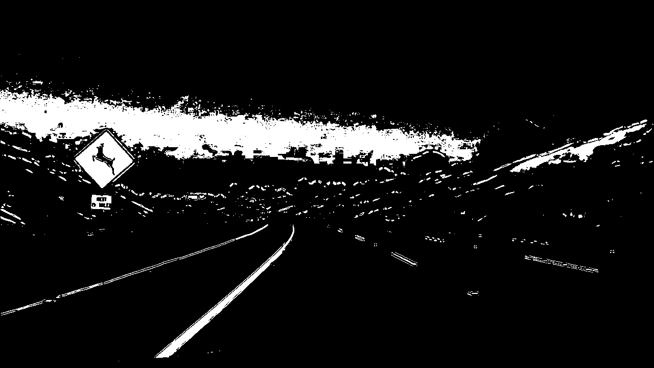 |
Figures show the camera image after applying distortion correction and thresholded image after applying the combined thresholds
3. Describe how (and identify where in your code) you performed a perspective transform and provide an example of a transformed image.
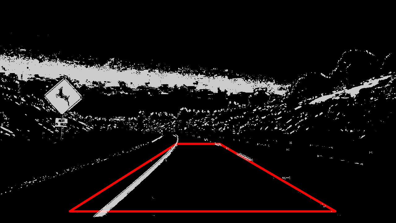
The code for perspective transform is built into the pipeline and uses an hardcoded source (src) and destination (dst) matrix.
src = np.float32([[570,464],[710,464],[1084,682],[225,682]])
offset = 200
dst = np.float32([[offset, 0], [img_size[0] - offset, 0], [img_size[0] - offset, img_size[1]], [offset, img_size[1]]])
This resulted in the following source and destination points:
| Source | Destination |
|---|---|
| 570, 464 | 200, 0 |
| 710, 464 | 1080, 0 |
| 1084, 682 | 1080, 720 |
| 225, 682 | 200, 720 |
To apply perspective transform, the 'M' matrix is first computed using M = cv2.getPerspectiveTransform(src, dst)
Similarly the Minv is also computed by swapping the src and dst matrices.
To warp an image the 'M' matrix is used with function cv2.warpPerspective
Lines 272 through 279 in my code perform the perspective transform
| Source Points Overlayed | After applying Perspective Transform |
|---|---|
 |
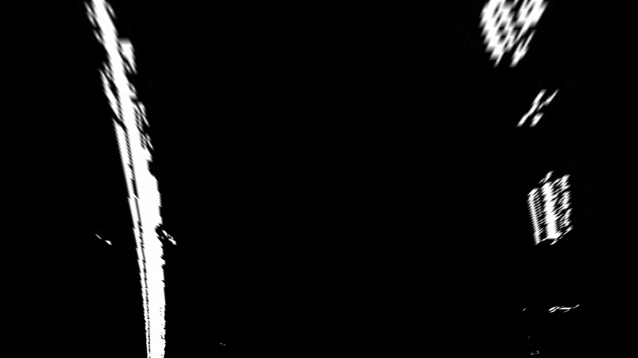 |
Figures show the bounding box used as source points and the resultant image after performing perspective transform
4. Describe how (and identify where in your code) you identified lane-line pixels and fit their positions with a polynomial?
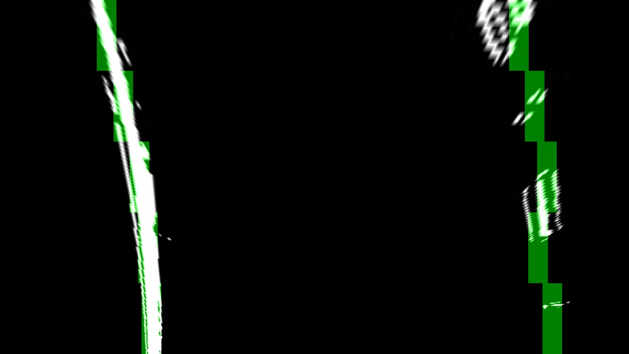
The convolution method is used here to identify the lane lines.
Function find_window_centroids from line 201 thru 236 performs the image slicing, convolution to find the lane hotspots.
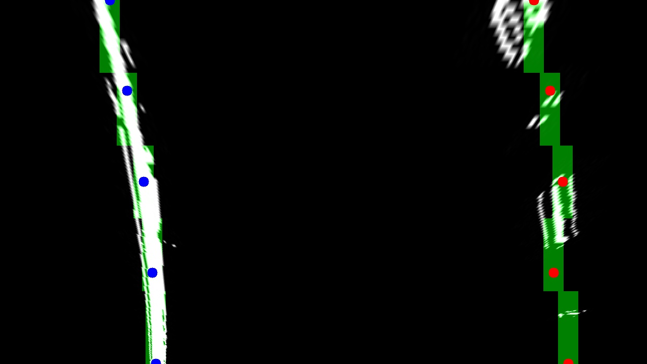
The identified region is stored in left and right point matrices which are then used to perform a curvefit using np.polyfit of 2nd order.
| Original Warped Image | Hot spots from the warped Image |
|---|---|
 |
 |
| Centers of the regions of interest | Curvefitted line through the points |
 |
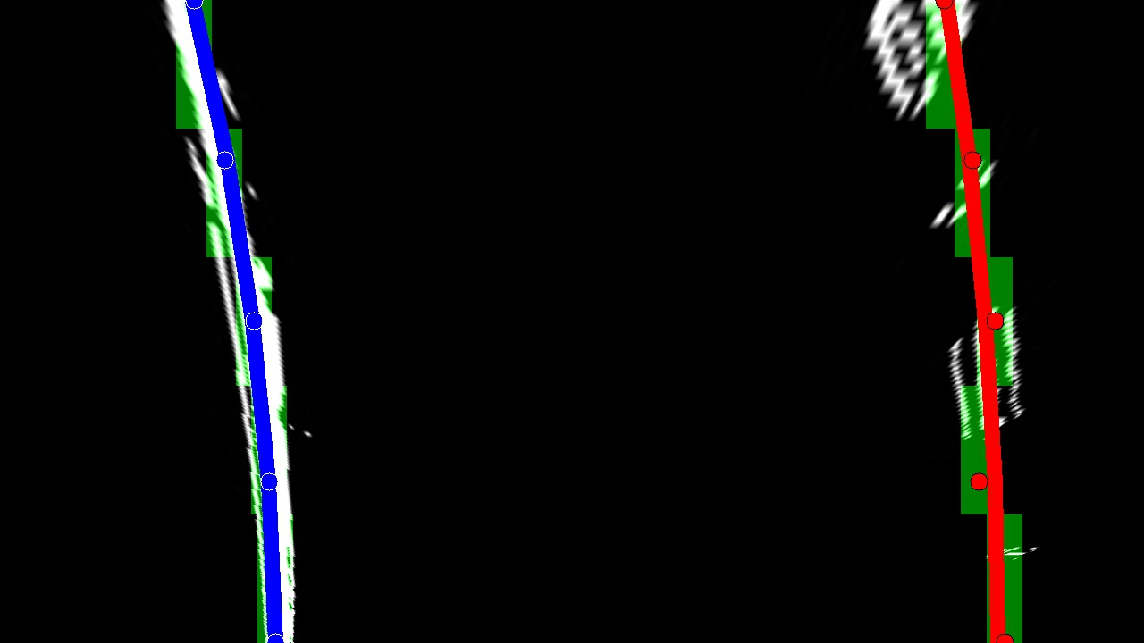 |
*Figures show the warped image, output of sliding window search using convolution, centers of the hotspots and curvefitted lines *
5. Describe how (and identify where in your code) you calculated the radius of curvature of the lane and the position of the vehicle with respect to center.
Based on US road regulations (3.7 meter wide minimum lane width) and from a sample image the lane section is approximately 30 m long, the pixel to real world conversion factors are calculated. Lines 355 through 364 show the radius of curvature implementation.
ym_per_pix = 30/720 # meters per pixel in y dimension
xm_per_pix = 3.7/700 # meters per pixel in x dimension
The polynomials are then fit to real world x and y dimensions (line
# Fit new polynomials to x,y in world space
left_fit_cr = np.polyfit(ploty*ym_per_pix, leftx*xm_per_pix, 2)
right_fit_cr = np.polyfit(ploty*ym_per_pix, rightx*xm_per_pix, 2)
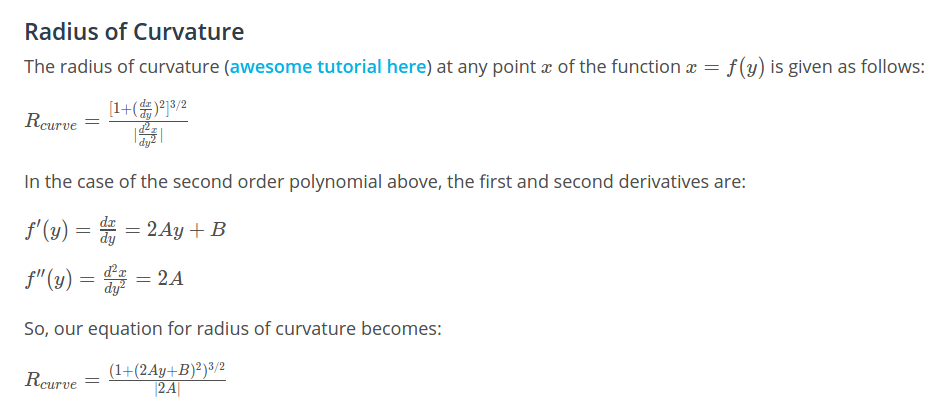 Formula for calculating radius of curvature[3]
Using above formula the lane curvature radius is calculated and displayed on the resultant image in meters.
Further, the left and right points detected from the convolution based window search are then used to fit left and right lane lines. The car position is known at the center of the camera. The average of the left and right lane lines gives the center of the lane. The car position and center lane position is then subtracted and multiplied by the pixel to real world conversion factor to obtain the relative position of the car w.r.t. center of the lane in meters.
6. Provide an example image of your result plotted back down onto the road such that the lane area is identified clearly.
The curvefitted lane lines are then highlighted by plotting a polygon using cv2.fillPoly
The resultant image is then unwarped using the Minv matrix and using cv2.warpPerspective function
The calculated lane curvature and relative vehicle position is then displayed at the corner of the image using cv2.putText
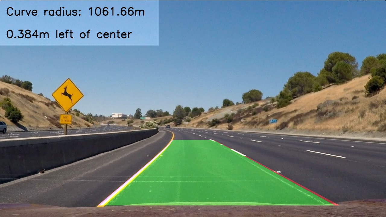 Figure shows the processed image after drawing the polygon and displaying the curvature, position
| Original Project Video | Processed Project Video |
|---|---|
 |
 |
1. Briefly discuss any problems / issues you faced in your implementation of this project. Where will your pipeline likely fail? What could you do to make it more robust?
The camera calibration is performed in at first to calculate the distortion correction factors. The distortion correction code is implemented at the very beginning of the pipeline so that all images are corrected for distortion. The Sobel operator is used in X, Y, Magnitude, Direction along with S channel and V channel thresholding. Further, these thresholding techniques are combined to obtain an image with minimal unnecessary information. Perspective transform is then used to obtain 'birds eye view' of the lane in front of the car. The transformed image is then processed through a sliding window search code which uses convolution to identify the lane lines. The identified hot spot points are then used to perform a polynomial curvefit of 2nd order to obtain a smooth lane line. This lane line is then unwarped using Perspective Transform along with lane section highlighting. The radius of lane curvature is calculated using the R_curve formula. The vehicle relative location is then calculated using center of lane and center of the camera calculation.
Shortcomings
- The thresholding is limited to given lighting situation
- The perspective transform calculation is performed using hardcoded source and destination points. The transformation matrix may not work very well for steep curves.
- The combination of these techniques may not work very well in harsh climate (heavy rain, snow etc.)
- The current pipeline does not perform sanity checks, if the actual lane lines are blocked for some reason, the code may return garbage lane lines.
[1] Lesson 22 Magnitude of the Gradient - Project: Advanced Lane Finding
[2] Lesson 23 Direction of the Gradient - Project: Advanced Lane Finding
[3] Lesson 35 Measuring Curvature - Project: Advanced Lane Finding