Video summarization is downsizing a video into a few related and important keyframes. Video, in essence, can be seen as a collection of frames, temporally related to one another. Seen this way, video summarization is a lossy compression of an input video, producing a few keyframes that viewers can skim rapidly to rapidly overview the video content.
Given a raw video file without any information of Intra-Frames (I-Frames), we approach this problem in 3 steps:
- Keyframes Extraction
- Keyframes Importance Ranking
- Keyframes Blending
Keyframes are similar to I-Frames. They are the initial frames in a scene that is selected in such a way that the remaining frames in a particual scene can be encoded more efficiently with less entropy. Following this definition, a scene consists of this initial frame (keyframe) and the remaining frames for that scene. Our goal in this step is to extract these keyframes. Unlike video encoders which must maintain strict temporal relationship between keyframes and compressed frames (either P- or B- frames), our keyframes extraction does not have this constraint.
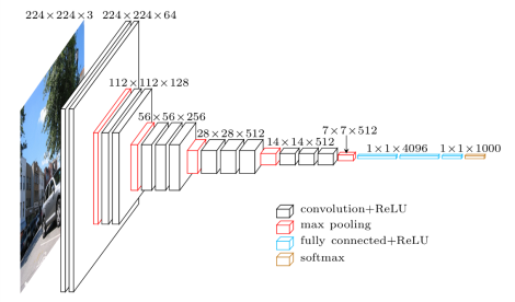
Our experience in computer vision lead us to not work at pixel-level directly. We instead opted to use feature-space output of VGG19 neural network trained on ImageNet dataset. All frames are thus feed-forwarded to the VGG19 network. We then store the output from the last max-pooling layer in-memory for further processing. See VGG19 Feature Extractor[1] for visual examples of these features in action.
Now we have an array of Features in size of (T * W * H), where T is the number of frames in the video, W and H are width and height in pixels respectively. Our next goal is to identify scenes. We use a First-Order Differentiator (FOD). FOD's task is to identify abrupt changes. This can be accomplished easily by linear single-pass scan throughout the Features, comparing two successive frames and recording their Cosine Difference. Abrupt changes in visual Feature is indicated by high value close to 1. We use a combination of adaptive algorithm and timeframe constraint to determine the threshold for FOD. This adaptive algorithm adjusts Cosine Distance threshold dynamically so that fast-paced scenes and slower, gradually changing ones can be detected equally accurately. We also impose a timeframe constraint that prevents scene creation below a certain number of frames in rapidly changing scenes. Consequently, the constraint also mandates scene separation when adaptive algorithm fails to detect new scene after a certain number of frames.
Frames produced by FOD are then marked as keyframes, which creates separation between scenes. We then perform cross-correlation of these keyframes based on their Cosine Distance. A typical FOD result looks like the heat map below, with lighter colors indicate similar frames and darker colors indicate different frames.
FOD may detect blank, dark scene as keyframes. We need to remove such frames. To do so, we convert all frames to HSL colorspace. We take the mean and standard deviation of Luminance from all frames and remove those with average Luminance two standard deviations below mean. This is the only part of the algorithm that works at pixel-level.
FOD is a coarse method in determining scenes. It has advantage in speed due to its single-pass, non-windowing method in detecting scene change. The disadvantage is obvious, FOD may not recognize scene separation in gradual changes. To detect this, we have the Second Pass Analysis (SPA).
SPA analyzes each scene independently and performs cross-correlation of the frames inside that particular scene by their Cosine Distance. SPA then attempts to detect clustering by iteratively running Principal Component Analysis (PCA). SPA increases PCA's number of clusters until it can capture 80% of the variance in the scene. This number is derived empirically through experiments. Knowing the number of appropriate clusters allows us to subdivide the scene into smaller ones, effectively inserting new separating keyframes. If we have more than one clusters, FOD must have missed the scene change.
A typical smooth scene with steady motion looks like the following
A scene with alternating scenes looks like the heatmap below. In this case, SPA detects that 2 clusters are needed to capture 80% variance in the scene.
Thus, a new keyframe is inserted. For reference, the keyframes extracted from the video look like the figure below. It is obvious (to human) that there is a scene change, yet FOD missed it.
With the new keyframes, it is possible that we have generated similar keyframes resulting in overpopulation. A typical output from SPA looks like the following:
Unlike video encoders that must maintain temporal constraints between I-Frames, Keyframe Extraction do not need the non-distinct keyframes. We can discard similar keyframes by voting and statistical process. First, we cross-correlate the Cosine Distance from all keyframes at this point. Then we take the mean and standard deviation. Frames which have Cosine Distance two standard deviations below the mean are moved to the elimination pool. Then each remaining keyframes "vote" which of the frames in the elimination pool stay by selecting a frame with the highest Luminance value. This voting process is necessary because keyframes similarity has many-to-many relationship property. The final result of Keyframe Extraction is visualized in the heat map below.
The keyframes extracted are then arranged hierarchically based on their importance. We selected 4-level of importance. Rank-0 are the few, most important frames. We trained a shallow 3-layers neural network with supervised training method. The features are temporal relationships, COCO[2] object detection, and average HSL values. We provided ground truth keyframes labeled with importance rank and we let the network to derive the weights and biases to each features.
Temporal relationships is 1-by-24 matrix that contains the Cosine Distance of a particular keyframe to 12 keyframes preceding and 12 keyframes succeeding it. The network will learn the importance weight based on the similarity of keyframes. For example, similar keyframes that appear successively will have lower importance. This phenomena is common in handheld or head-mounted camera, where involuntary camera movement may create unnecessary scene changes.
COCO object detection provides information of 80-classes object recognition. Hence, the size is 1-by-80 matrix. We use YOLO[3] to extract objects and their bounding boxes. Based on the bounding boxes, we can derive the area of each object relative to the frame size. If there are multiple objects of a particular class, we simply take the largest bounding boxes. These area information are then multiplied with the highest detection confidence to populate the 1-by-80 matrix. This maximizing process is used instead of accumulation so that a single object, occupying large portion of the screen, generates higher importance compared to many, smaller objects.
Average HSL values are used based on observation that human are more attracted towards a certain hue (e.g. natural skin color, wooden, warm-lit environment). Luminance within a certain range, as well as saturation, may also play important role. This is a 1-by-3 matrix that the network needs to figure out the weight based on the provided ground truth.
The equation can then be simplified as X * W = Y, where
-
X is a [1-by-107] feature matrices
-
W is a [107-by-4] weights and biases that the network need to figure out
-
Y is a [1-by-4] importance rank, provided as labeled ground truth during training and generated during testing
The shallow network uses categorical crossentropy loss function. Metric used is accuracy. We believe this metric is not an optimal choice. We should penalize less if the importance difference is minimal (e.g. rank-2 identified as rank-3 or vice versa) and penalize heavily otherwise. We used Adam optimizer with very low learning rate at 0.01. The network consists of 3 layers:
- Fully-connected layer with 107 input neurons and 16 output neurons
- A simple dropout layer at 20% probability
- Fully-connected layer with 16 input neurons and 4 output neurons
We ran the training for 100,000 epochs, resulting 96% accuracy in trainset and 64% in testset at 10% train-test split. This is a clear indication of overfitting. This may have been caused by insufficient training data as we only have 25 minutes of training video, which is then split 10% for testing.
Once we have all the key frames, we need to arrange them (in a chronological order) to form a tapestry. The naive approach is to join the frames. For example:
To blend the keyframes further we can remove the most obvious colors like the black top and bottom borders. For example:
Both the above approaches do not form a tapestry but rather a larger image formed by joining other images (not blending). We can change this by performing seam carving on this larger image to try and blend them. In seam carving, our goal is to remove unnoticeable pixels that blend with their surroundings. Hence the energy is calculated by sum the absolute value of the gradient in both x direction and y direction for all three channel (B, G, R). Energy map is a 2D image with the same dimension as input image. We then delete the seam with the lowest energy. The output after seam carving is as follows:
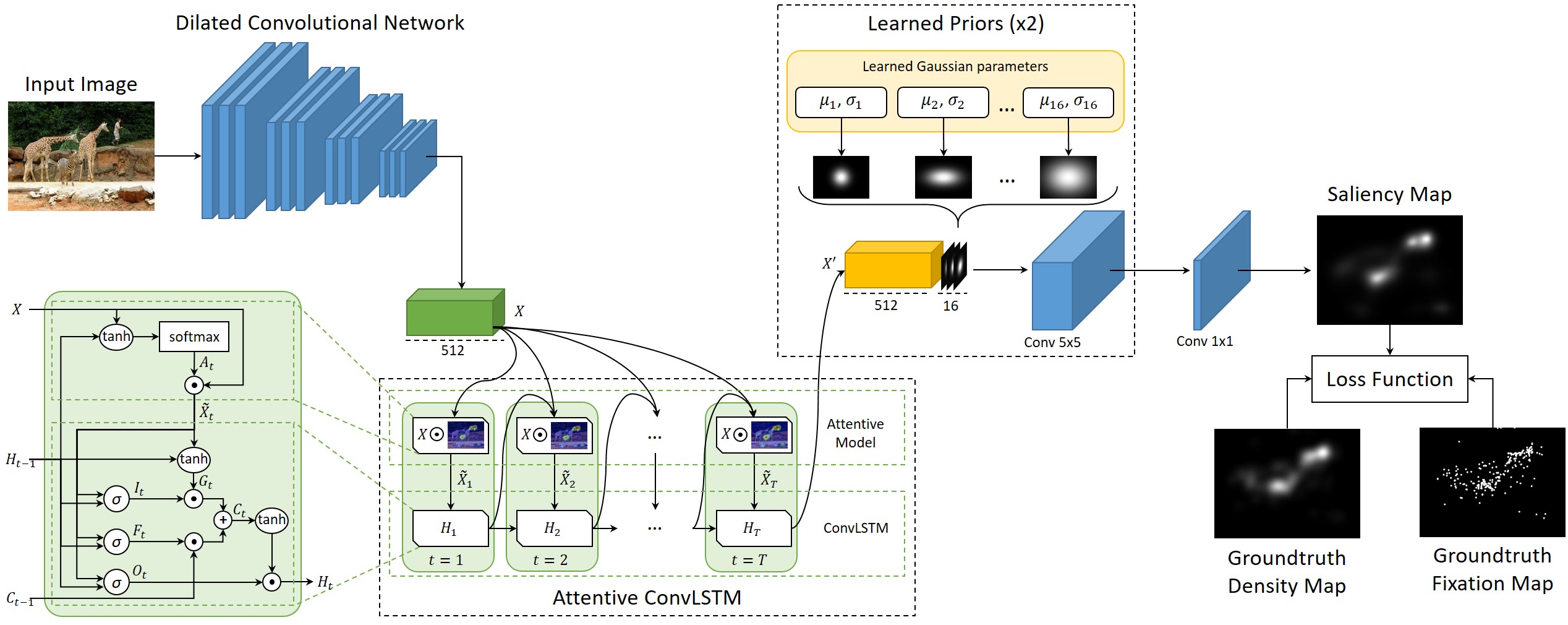
In the above seam carved image, you can see that some of the important objects have been distorted. This is because we haven't mentioned explicitly that those objects are important. Furthermore, how do we identify important objects? We define importance of an object based on human eye fixations. To predict human eye fixation in a frame we use a LSTM-based Saliency Attentive Model.
For example,
INPUT
OUTPUT
MASK created from output after thresholding (Threshold value is 50)
This neural network gives us a saliency map which can be used as a mask (after thresholding) in the seam carving process. The energy values in the masked area will be multiplied by a very high constant value so it never has a low energy value and hence that seam won't be selected. The output of seam carving with masking:
- VGG19 Feature Extractor VGG19 Feature Extractor
- Common Object in Context COCO
- YOLO YOLO
- Predicting Human Eye Fixations via an LSTM-based Saliency Attentive Model SAM
- Seam Carving for Content-Aware Image Resizing seam carving


