QM/MM Modelling of Enzyme Reactions
Aimed at:
Anyone interested in starting to use QM/MM simulations for their research, in particular for enzyme reactions.
Requirements:
Basic knowledge of the Linux command line.
Abstract:
The training workshop will introduce non-specialists to the use of combined quantum mechanics/molecular mechanics (QM/MM) methods for modelling enzyme-catalysed reaction mechanisms. Concepts and techniques of QM/MM reaction modelling will be explained through hands-on exercises. During the tutorial, each participant will generate and analyse a free energy profile and a potential energy profile for the reaction catalysed by chorismate mutase.
Training Material
The tutorial workshop consists of a series of scripts to run the simulations and analysis of the outputs, accompanied by an informal lecture. The scripts can be run using the CCPBioSim training server.
Once you have started the server open a Terminal (Click "New" top-right of the item list, and choose "Terminal" from the list). You will find the scripts and all other required workshop files there. Once you are finished, please use the "logout" button on the jupyter server page (top right).
All material was prepared by Marc van der Kamp with assistance from Sam Johns.
Contents
In this tutorial workshop, you will learn how to apply combined quantum mechanics/molecular mechanics (QM/MM) methods to model a chemical reaction in an enzyme. You will calculate a free energy profile and a potential energy profile for the reaction, and analyse an important interaction in the active site.
You will be using the simulation software from the AmberTools package. The sander programme is capable of the QM/MM simulations required. For efficiency, the semi-empirical QM method PM6 will be used throughout (implemented directly in sander). You can further use VMD to visualise the simulations on your local machine (after downloading the final files).
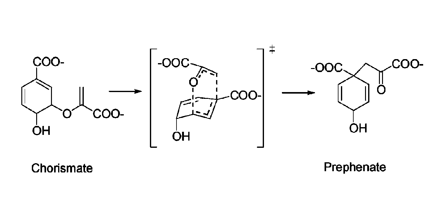
You will be simulating the enzyme-catalysed reaction of chorismate to prephenate. This is an intramolecular reaction. The reaction proceeds via a cyclic transition state. A (geometric) reaction coordinate can be defined as the difference between the length of the C-O bond that is breaking, and the length of the C-C bond that is forming. Plotting the energy of the molecule as a function of this reaction coordinate returns a reaction energy profile.
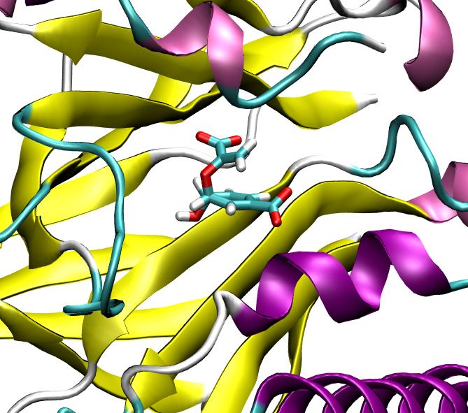
This reaction is catalysed by the enzyme chorismate mutase. Chorismate mutase helps catalyse the conversion of chorismate to prephenate by lowering the activation energy of the reaction. The enzyme-substrate (chorismate) complex has been set up for simulation using the X-ray crystal structure 2CHT (first trimer) and the Enlighten tools.
NB: Whenever text is written in a box like this, it is a command that should be typed on the command line of the terminal, or a reference to a file/directory.
Calculating a free energy profile using umbrella sampling
We will simulate the reaction starting from a 'snapshot' from a standard MM dynamics simulation (generated using the Enlighten DYNAM protocol). You can choose your own starting structure from the md*.rst files available in the qmmm-workshop directory (md1.rst to md20.rst).
Preparation
Make a new directory inside it and add a symlink (symbolic link or soft link) entitled md.rst to the starting structure of your choice. For example for starting structure md5.rst:
NB: Please choose your own, different, starting structure - replace 5 with a number between 1-20.
mkdir us5
cd us5
ln -s ../data/md5.rst md.rst
To set up umbrella sampling, you can use the bash-script setup_umb_samp.sh as follows:
bash ../scripts/setup_umb_samp.sh
You will notice that a range of sub-directories has been generated, one for each "umbrella sampling window", spaced 0.15 Ang apart along the reaction coordinate for the reaction (see above). Inside these directories there is a sander input file for a short (1 ps) QM/MM simulation, md1ps.i, with a restraint on the reaction coordinate value (defined in the .RST file).
Running umbrella sampling
The setup_umb_samp.sh script also generated a new script, run_umb_samp.sh. This contains the commands to run the umbrella sampling simulations sequentially, from the substrate complex (in rc-1.80) to the product complex (in rc1.80). To run the simulations in the 'background', type:
bash run_umb_samp.sh &
(See instructions in the script to run this through a PBS queing system instead, in case you are not running this on the CCPBioSim workshop server.)
Now, the first umbrella sampling simulation should start, and you will see new files written in the directory rc-1.80. Values of the reaction coordinate at each simulation step (1 fs) are collected in rc-1.80/rc-1.80_1.tra.
Running these umbrella sampling simulations will take a little while (~25 minutes).
While you are waiting, you can download the wt.sp20.top file and the restart file you selected (e.g. md5.rst) to your PC and load & view in VMD. See further below, Visualising the umbrella sampling simulation in VMD.
You can continue with the next part of the tutorial, Calculating a potential energy profile using sequential QM/MM minimisations, once the umbrella sampling window with reaction coordinate value -0.3 has finished, i.e. rc-0.30/rc-0.30_1.tra is complete (1000 lines), which should take ~10-12 minutes.
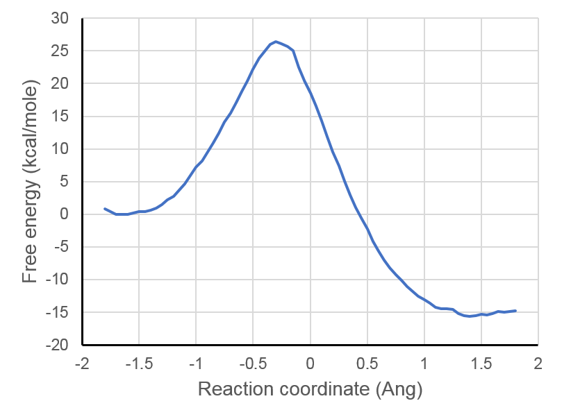
Analysis: the free energy profile for the reaction
To obtain the free energy profile or PMF (potential of mean force) for the reaction you simulated using umbrella sampling, we will use the Weighted Histogram Analysis Method (WHAM). Before we can do this, all umbrella sampling windows must be finished.
To run WHAM, type:
bash ../scripts/run_wham.sh
This will take a few seconds and generate a 'metafile', meta.dat, and use this to run the WHAM code. The WHAM code then generates wham.log and wham.txt. The first line of wham.log shows the command that was used to run WHAM. the wham.txt file contains the results.
To plot the free energy profile, download wham.txt (navigate to your umbrella sampling directory in the Jupyter window and tick the box next to the file and click the Download button above the file listing).
Import in your favourate plotting program (e.g. Excel).
Alternatively, copy and paste column-by-column from the terminal window to your plotting program, e.g. after using:
sed /^#/d wham.txt | cut -f 1
sed /^#/d wham.txt | cut -f 2
Once you have imported the data, plot the first column on the x-axis and the second on the y-axis.
Note that the WHAM program has (arbitrarily) set free energy of the bin with lowest free energy value to zero. You can make a third column where you set the reactant complex minimum to zero instead.
(See the 'umbrella sampling' sheet in qmmm-workshop/example/example.xls.)
Note that because the simulations that were run were rather short (1 ps per window), it is unlikely that the free energy profile is converged.
Visualising the umbrella sampling simulation in VMD
To aid visualisation of the series of simulations, first create a trajectory of the sequential umbrella sampling simulations (once it has finished completely):
$AMBERHOME/bin/cpptraj < ../data/make_us_trj.in &> make_us_trj.log
Download the generated trajectory us_traj.mdcrd and wt.sp20.top (located in qmmm-workshop) to your PC and load & view in VMD as follows:
- Go back to the initial Jupyter notebook tab (File browser) and navigate to files. To download files, tick the box next to the file and click the Download button above the file listing.
- Start VMD.
- In the main VMD menu, choose: File --> New Molecule.
- Select
wt.sp20.topand set filetype as "AMBER7 Parm". Then press "Load". - Browse to trajectory: us_traj.mdcrd. Set filetype as "AMBER Coordinates". Press "Load".
- Select
- In the main menu, choose: Graphics --> Representations.
- Create representations, e.g. "all" with Drawing Method "NewCartoon" and "resname CHO" with Drawing Method "DynamicBonds".
Note how the bond lenghts of the C-O bond that is broken and the C-C bond that is formed change along the trajectory.
Calculating a potential energy profile using sequential QM-MM minimisations
We will obtain a potential energy profile of the reaction starting from a 'snapshot' from the umbrella sampling simulation around the transition state of the reaction. The chorismate-to-prephanate reaction in chorismate mutase has a transition state around the reaction coordinate value of -0.30. We can therefore start once the umbrella sampling window with reaction coordinate value -0.3 has finished, i.e. rc-0.30/rc-0.30_1.tra is complete.
To obtain the potential energy profile, sequential QM/MM energy minimisations will be used, with a (strict) restraint on the reaction coordinate values. The QM/MM energy will thus be obtained for different values of the reaction coordinate. To ensure a change in the structure that is not directly related to the reaction occurs (which may cause a 'discontinuity' in the energy profile), positional restraints will be applied to residues and water molecules that do not have any atom within 5 Ang of the reacting molecule. This approach can be referred to as adiabatic mapping.
In addition to obtaining the potential energy profile, we will also:
- calculate the energy of the reacting molecule along the potential energy profile without the enzyme present (using 'single point' calculations in the gas-phase with the AmberTools program sqm)
- calculate the energy of the enzyme-reacting molecule complex along the potential energy profile without a key residue, Arg90 in the original numbering (using 'single point' calculations in sander, after 'stripping' away the Arg90 side-chain with cpptraj).
Preparation
Create a new directory, e.g. called adiab5 (if you originally started with md5.rst), for running the 'adiabatic mapping', move into it:
NB: In all the below example commands, please replace 5 with the number you chose previously (between 1-20).
cd ..
mkdir adiab5
cd adiab5
Once the umbrella sampling has finished running for reaction coordinate value -0.3, make a symlink to the restart file for this umbrella sampling window (e.g. ../us5/rc-0.30/:
ln -s ../us5/rc-0.30/md1ps.rst md1ps_rc-0.3.rst
Perform 'adiabatic mapping' and single point calculations
For efficiency, all the steps required to perform the aforementioned energy minimisations for 'adiabatic mapping' and the single-point calculations are included in a single script, run_adiab_all.sh.
Note that this script also creates a system with a periodic box of water molecules (as opposed to the sphere of water molecules that was used during umbrella sampling, for efficiency). This is because the minimisation algorithms available in sander that are required for 'adiabatic mapping' (specified by the xmin=3 option) do not work properly without a periodic box definition.
To run the script (in the background), simply type:
bash ../scripts/run_adiab_all.sh &
This should take about ~7-10 minutes in total.
For more information about the different steps that are performed in the script, read the comments in the run_adiab_all.sh script (e.g. by opening it in nano).
Once the script has finished, the energy values obtained will be written to the file adiabatic_mapping_energies.dat.
Analysis: the potential energy profile and single point calculations
To plot the potential energy profile and the related single point calculations, download adiabatic_mapping_energies.dat (navigate to your umbrella sampling directory in the Jupyter window, tick the box next to the file and click the Download button above the file listing).
Import this file in your favourate plotting program (e.g. Excel).
Alternatively, copy and paste column-by-column from the terminal window to your plotting program, e.g. using:
cut -f 1 adiabatic_mapping_energies.dat (the reaction coordinate values for which energies were calculated)
cut -f 2 adiabatic_mapping_energies.dat (the total QM/MM energies of the potential energy profile)
cut -f 3 adiabatic_mapping_energies.dat (the single-point QM energies of the reacting species along the potential energy profile)
cut -f 4 adiabatic_mapping_energies.dat (the single-point QM/MM energies of the potential energy profile excluding the Arg90 side-chain)
Once you have imported the data, make additional columns with the energies relative to the enzyme-substrate minimum energies (by subtracting value of minimum energy, likely at reaction coordinate value -1.4) for each of the three cases and plot against reaction coordinate value.
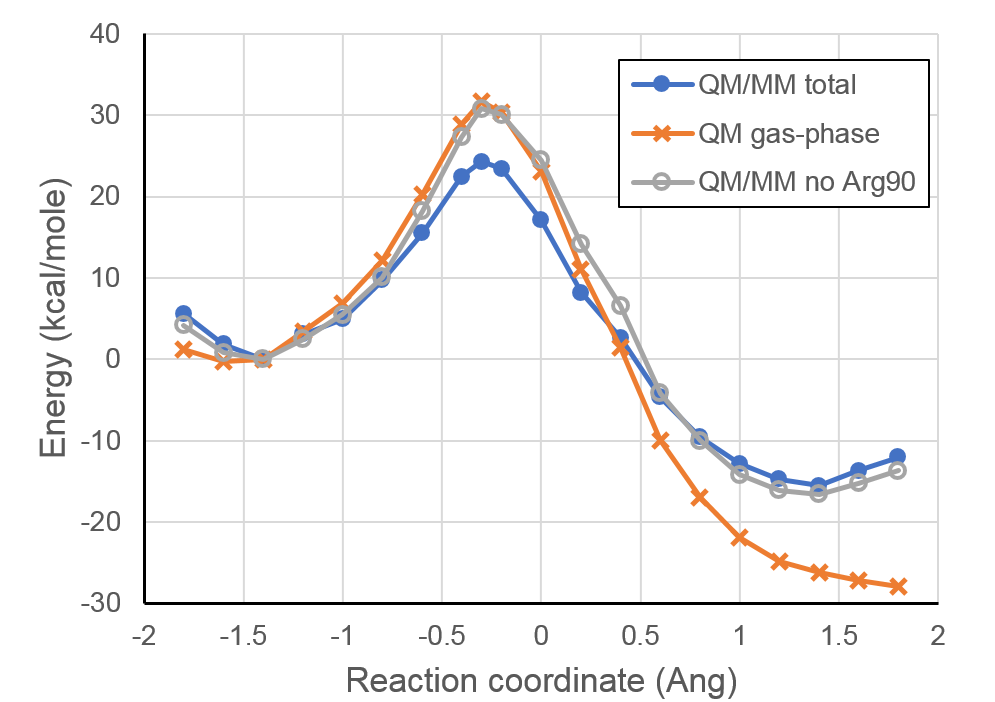
The plot should look something like this:

(See the 'adiabatic mapping' sheet in example/example.xls.)
Note how:
- the enzyme environment lowers the barrier to reaction (i.e. stabilises the energy of the transition state complex), compared to the 'gas-phase' energies
- the enzyme environment 'destabilises' the product complex (again compared to the 'gas-phase energies')
- the enzyme environment without the Arg90 side-chain does not contribute much to the stabilisation of the transition state. In other words: the main stabilisation is due to Arg90.
Visualising the 'adiabatic mapping' simulation in VMD
To aid visualisation of the structures along the potential energy profile, first create a trajectory of the sequential energy minimisations (once run_adiab_all.sh has finished completely):
$AMBERHOME/bin/cpptraj < ../adiab/make_adiab_trj.in &> make_adiab_trj.log
Download the generated trajectory adiab_traj.mdcrd and wt.box.top to your PC and load & view in VMD as follows:
-
Go back to the initial Jupyter notebook tab (File browser) and navigate to files. To download files, tick the box next to the file and click the Download button above the file listing.
-
Start VMD.
-
In the main VMD menu, choose: File --> New Molecule.
- Select
wt.box.topand set filetype as "AMBER7 Parm". Then press "Load". - Browse to trajectory: adiab_traj.mdcrd. Set filetype as "AMBER Coordinates with Periodic Box". Press "Load".
- Select
-
In the main menu, choose: Graphics --> Representations.
-
Create representations, e.g. "all" with Drawing Method "NewCartoon" and "resname CHO" with Drawing Method "DynamicBonds".
-
If you have already set up representations for the trajectory from umbrella sampling, you can also 'Clone' these. In the main VMD menu, choose: Extensions --> Visualization --> Clone Representations.
-
To show the Arginine residue that is key for transition state stabilisation, you can create a representation with e.g. e.g. "resid 203" (original residue Arg90, in the third chain of the trimer) with Drawing Method "Licorice"
Again, you can see how the bond lenghts change of the C-O bond that is broken and the C-C bond that is formed. Further note the difference between the umbrella sampling MD simulations and the 'adiabatic mapping' energy minimisations. Does the positioning of Arg90 make sense, in light of its role in transition state stabilisation?
Example output and visualisation
If, for any reason, you encounter problems with completing the simulations and visualising them in VMD, you can load example trajectories for umbrella sampling and adiabatic mapping as follows:
Download wt.sp20.top from the top directory, and us_traj.mdcrd, wt.box.top, adiab_traj.mdcrd and view_traj.vmd from the directory example to the same location on your local PC (which should have VMD installed).
Open VMD and in the command line window (window name ending in vmd.exe in Windows OS), change directory to the location you downloaded the files, for example:
cd O:/Downloads/
Then, from the VMD Main window, do File --> Load Visualization State... and choose view_traj.vmd.
This should load the umbrella sampling simulation in the "Molecule" wt.sp20.top and the adiabatic mapping simulation in the "Molecule" wt.box.top. You can now turn off the view of one of these by double-clicking on "D" in front of the molecule name in the VMD Main window, double-click on "T" in front of the molecule you are viewing, and press the play button to view the simulation.
Final comments
Note that the simulation setup, QM method and protocols used here are mainly optimised for speed, NOT accuracy.
If you are interested in the actual steps and commands required to generate the simulations and results in this tutorial, please take a look at the shell scripts (e.g. run_adiab_all.sh, setup_umb_samp.sh), which are commented.
The protocols demonstrated in this workshop, with semi-empirical QM methods, are particularly relevant to enzyme reactions that do not involve (transition) metals or radicals etc. For tutorial material involving QM/MM enzyme reaction modelling with transition metals (Cytochrome P450), please see the CCPBioSim ChemShell QM/MM workshop. This site also contains useful practical information for QM/MM calculations in enzymes.
Further reading
Reviews
Van der Kamp MW & Mulholland AJ. Combined quantum mechanics/molecular mechanics (QM/MM) methods in computational enzymology Biochem. (2013) 52, 2708-2728. DOI
Senn HM & Thiel W. QM/MM Methods for Biomolecular Systems Angew. Chem. Int. Ed. (2009) 48, 1198-1229. DOI
Lonsdale R, Harvey JN, Mulholland AJ. A practical guide to modelling enzyme-catalysed reactions Chem. Soc. Rev. (2012) 41, 3025-3038. DOI
Related publications on Chorismate Mutase QM/MM simulations
F. Claeyssens, K.E. Ranaghan, F.R. Manby, J.N. Harvey & A.J. Mulholland, 'Multiple high-level QM/MM reaction paths demonstrate transition-state stabilization in chorismate mutase: correlation of barrier height with transition-state stabilization'. Chem. Commun. 5068-5070 (2005). DOI
F. Claeyssens, K.E. Ranaghan, N. Lawan, S.J. Macrae, F.R. Manby, J.N. Harvey, A.J. Mulholland. 'Analysis of chorismate mutase catalysis by QM/MM modelling of enzyme-catalysed and uncatalysed reactions.' Org. Biomol. Chem., (2011) 9, 1578-90. DOI
K.E. Ranaghan, L. Ridder, B. Szefczyk, W.A. Sokalski, J.C. Hermann & A.J. Mulholland 'Insights into enzyme catalysis from QM/MM modelling: transition state stabilization in chorismate mutase', Mol. Phys. (2003) 101, 2695-2714
K.E. Ranaghan, L. Ridder, B. Szefczyk, W.A. Sokalski, J.C. Hermann, and A.J. Mulholland 'Transition state stabilization and substrate strain in enzyme catalysis: ab initio QM/MM modelling of the chorismate mutase reaction' Organic and Biomolecular Chemistry (2004) 2, 968-980
K.E. Ranaghan & A.J. Mulholland 'Conformational effects in enzyme catalysis: QM/MM free energy calculation of the 'NAC' contribution in chorismate mutase' Chem. Commun. (2004) (10), 1238-1239.


