xxIRT: Item Response Theory and Computer-Based Testing in R

October 02, 2018

Installation
Introduction
Package Modules
Ending

Installation

To install a stable version from CRAN, call install.packages("xxIRT") in R console. To install the most recent version from GitHub, call devtools::install_github("xluo11/xxIRT") in R console (if devtools package has not been installed yet, install it first). To remove the installed package, call remove.packages("xxIRT") in R console.

Introduction

xxIRT is a R package designed to provide a suite of practical psychometric analysis and research tools and implement latest advancements in psychometrics (especially pertaining to computer-based testing). The package is organized into five modules:

IRT Models
Parameter Estimation
Automated Test Assembly
Computerized Adaptive Testing
Multistage Testing

Package Modules

IRT Models

3PL Model

The 3-parameter-logistic (3PL) model was introduced by Birnbaum[1]. This model uses three item parameters (a, b, and c) and one people parameter (θ) to describe the probabilistic relationship between an item and a person. The three item parameters are often referred to as the discrimination, difficulty and pseudo-guessing of an item. By default, the scaling constant D=1.702. When c=0, the model is reduced to the 2PL model. When a=1 and c=0, the model is reduced to the 1PL model. When a=1, c=0, and D=1, the model is mathematically equivalent to the Rasch model[2].

The following functions are available for the 3PL model:

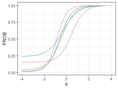
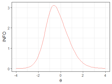
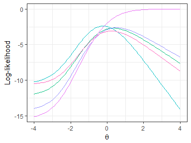
model_3pl_prob(t, a, b, c, D): Compute the probabilities of correct responses for given parameters. Return results in a people-by-item matrix. D=1.702 by default.
model_3pl_info(t, a, b, c, D): Compute the information for given parameters and return results in a matrix
model_3pl_lik(u, t, a, b, c, D, log): Compute the response likelihoods for given response data and parameters. Use log=TRUE to return log-likelihood.
model_3pl_rescale(t, a, b, c, param, mean, sd): Transform parameters to a new scale and return a list of rescaled parameters.
model_3pl_gendata(num_people, num_item, ...): Generate response data and parameters using the 3PL model. Pass in t, a, b, and c to fix parameters. Otherwise, draw these parameters from the normal, log-normal, normal and beta distributions respectively. Use t_dist, a_dist, b_dist, and c_dist to set the sampling distribution. Use missing argument to add missing response data.
model_3pl_plot(a, b, c, D, type, total, ...): Plot the item characteristic curves (ICCs; type='prob') or the item information function curves (IIFCs; type='info'). When total=TRUE, results are summed over items into test characteristic curve (TCC) or the test information function (TIF) curve.
model_3pl_plot_loglik(u, a, b, c, D, ...): Plot each person's log-likelihood functions. Use show_mle=TRUE to print a rough maximum likelihood estimate for each response vector.

Examples

# generate 1PL data with 10% missing
x <- model_3pl_gendata(10, 5, a=1, c=0, missing=.1)
# generate 3PL data and sample theta from N(.8, .5) and c-parameter from beta(1, 4)
x <- model_3pl_gendata(10, 5, t_dist=c(.8, .5), c_dist=c(1, 6))
# compute the probability using the Rasch model
p <- model_3pl_prob(x$t, 1, x$b, 0, D=1)
# compute the probability using the 3PL model
p <- model_3pl_prob(x$t, x$a, x$b, x$c)
# compute the information using the 3pl model
i <- model_3pl_info(x$t, x$a, x$b, x$c)
# compute the log-likelihood
l <- model_3pl_lik(x$u, x$t, x$a, x$b, x$c, log=TRUE)
## rescale parameters to a new scale where theta ~ N(0, 1)
xx <- model_3pl_rescale(x$t, x$a, x$b, x$c, param="t", mean=0, sd=1)

Graphs

# ICC
model_3pl_plot(x$a, x$b, x$c, type="prob")

# TIF
model_3pl_plot(x$a, x$b, x$c, type="info", total=TRUE)

# log-likelihood
model_3pl_plot_loglik(x$u, x$a, x$b, x$c)

Generalized Partial Credit Model

The generalized partial credit model (GPCM) was introduced by Muraki[3][4]. GPCM extends IRT to model polytomous responses, where items have more than two score categories. There are two parameterization of this model: (1) an item-by-category matrix of b-parameter as the item-category parameters, or (2) a vector of b-parameters as the item difficulty parameters and an item-by-category matrix of d-parameters as the item category parameters (the final item-category parameters are computed as: b − d). Because guessing is usually difficult for polytomous items, c-parameter is absent in GPCM. Note because the difficulty of the initial category of an item (b_j1 or d_j1) does not change the probabilities of score categories of that item, it is usually arbitrarily set to 0.

The following functions are available for GPCM:

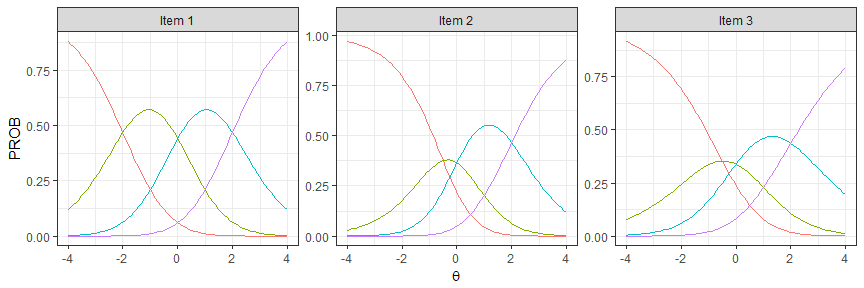
model_gpcm_prob(t, a, b, d, D, add_initial): Compute the probabilities of score categories for given parameters. When b is a matrix and d is NULL, b is used as the item-category parameter. When b is a vector and d is a matrix, b is used as the item difficulty parameter and d the item category parameter. Use add_initial to add the initial category to b or d. The scaling constant D=1.702 by default. The result is a 3-dimensional array: people by item by category.
model_gpcm_info(t, a, b, d, D, add_initial): Compute the information of score categories and return a 3D array as results.
model_gpcm_lik(u, t, a, b, d, D, add_initial, log): Compute the response likelihood and return a matrix as results. Use log=TRUE to return log-likelihood.
model_gpcm_gendata(num_people, num_item, num_category, ...): Generate response data and parameters using the GPCM. Pass in t, a, and b. Otherwise, draw these parameters from the normal, log-normal, and normal distributions respectively. Use t_dist, a_dist, and b_dist to set the sampling distribution. Use missing argument to add missing response data. Use set_initial to set the value of the initial category. If sort_b=TRUE, category difficulties are sorted for each item.
model_gpcm_plot(a, b, d, D, add_initial, type, by_item, total, xaxis): Plot the item category characteristic curves (ICCCs; type='prob') or item category information function curves (ICIFCs; type='info'). Use by_item=TRUE to combine category-level statistics into item-level statistics. Use total=TRUE to sum over items.
model_gpcm_plot_loglik(u, a, b, d, D=1.702, add_initial, xaxis, show_mle): Plot the log-likelihood for each response vector. Use show_mle to print a rough maximum likelihood estimate for each response vector.

Examples

# generate data: 10 peopel, 5 item, 3 categories in each item
x <- model_gpcm_gendata(10, 5, 3, set_initial=0)
# compute probability
p <- model_gpcm_prob(x$t, x$a, x$b, NULL)
# compute informtaoin
i <- model_gpcm_info(x$t, x$a, x$b, NULL)
# compute likelihood
l <- model_gpcm_lik(x$u, x$t, x$a, x$b, NULL)

Graphs

# Figure 1 in Muraki, 1992 (APM)
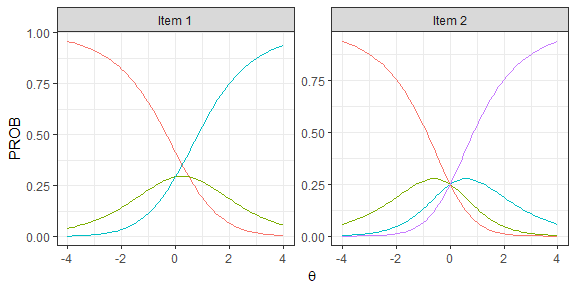
model_gpcm_plot(a=c(1,1,.7), b=matrix(c(-2,0,2,-.5,0,2,-.5,0,2), nrow=3, byrow=TRUE), d=NULL, D=1.0, add_initial=0, xaxis=seq(-4, 4, .1), type='prob')

# Figure 2 in Muraki, 1992 (APM)
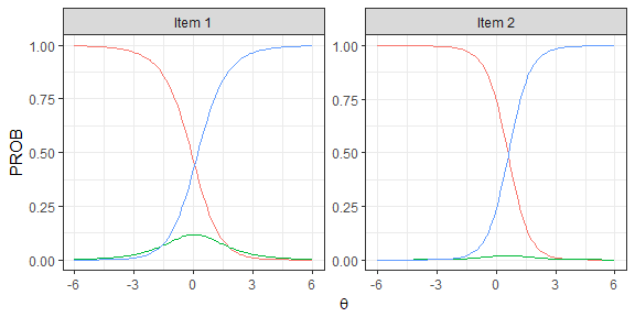
model_gpcm_plot(a=.7, b=matrix(c(.5,0,NA,0,0,0), nrow=2, byrow=TRUE), d=NULL, D=1.0, add_initial=0, xaxis=seq(-4, 4, .1))

# Figure 3 in Muraki, 1992 (APM)
model_gpcm_plot(a=c(.778,.946), b=matrix(c(1.759,-1.643,3.970,-2.764), nrow=2, byrow=TRUE), d=NULL, D=1.0, add_initial=0)

# Figure 1 in Muraki, 1993 (APM)
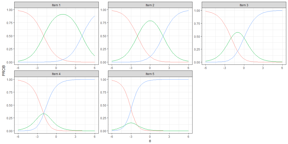
model_gpcm_plot(a=1, b=matrix(c(0,-2,4,0,-2,2,0,-2,0,0,-2,-2,0,-2,-4), nrow=5, byrow=TRUE), d=NULL, D=1.0)

# Figure 2 in Muraki, 1993 (APM)
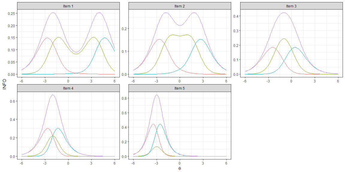
model_gpcm_plot(a=1, b=matrix(c(0,-2,4,0,-2,2,0,-2,0,0,-2,-2,0,-2,-4), nrow=5, byrow=TRUE), d=NULL, D=1.0, type='info', by_item=TRUE)

Parameter Estimation

Parameters are often unknown and need to be estimated using statistical procedures, and parameter estimation is a central activity in IRT. The following functions are available for the estimation of 3PL model:

model_3pl_jmle(u, t=NA, a=NA, b=NA, c=NA, D=1.702, num_iter=100, num_nr=15, h_max=1.0, conv=.1, decay=.95, scale=NULL, bounds=list(), priors=list(), debug=TRUE): A joint maximum likelihood estimator of θ and item parameters, and a MAP estimator when priors is set. Pass in t, a, b, c to fix parameters. Use num_iter and num_nr to control the maximum cycles of E-M iteration and Newton-Raphson iteration. Use conv to control the convergence criterion. The estimation terminates when the log-likelihood decrement is less than conv. Use scale to set the scale for θ. Use bounds and priors to control the bounds and priors of parameters. Use debug=TRUE to turn on the debugging mode.
model_3pl_mmle(u, a=NA, b=NA, c=NA, D=1.702, num_iter=100, num_nr=15, num_quad=c('11', '20'), h_max=1.0, conv=.1, decay=.98, scale=NULL, bounds=list(), priors=list(), debug=FALSE): A marginal maximum likelihood estimator of θ and item parameters. Item parameters are estimated first using the marginal distribution of θ, and θs are estimated afterwards.
model_3pl_eap_scoring(u, a, b, c, D): An EAP estimator of θs.

The following functions are available for the estimation of GPCM:

model_gpcm_jmle(u, t, a, b, d, D, set_initial, num_iter, num_nr, h_max, conv, decay, scale, bounds=list(), priors=list(), debug): A joint maximum likelihood estimator.

Examples

Generate data: 3000 people, 60 items

data_tru <- model_3pl_gendata(3000, 60)

Joint maximum likelihood estimation

data_est <- model_3pl_jmle(u=data_tru$u, scale=c(0, 1), priors=NULL)
evaluate_3pl_estimation(data_tru, data_est)

## Parameter t: corr=0.97, rmse=0.26
## Parameter a: corr=0.93, rmse=0.09
## Parameter b: corr=1, rmse=0.08
## Parameter c: corr=0.34, rmse=0.06

MAP with joint maximum likelihood estimation

data_est <- model_3pl_jmle(u=data_tru$u, scale=c(0, 1))
evaluate_3pl_estimation(data_tru, data_est)

## Parameter t: corr=0.97, rmse=0.24
## Parameter a: corr=0.94, rmse=0.09
## Parameter b: corr=1, rmse=0.07
## Parameter c: corr=0.61, rmse=0.03

Marginal maximum likelihood estimation

data_est <- model_3pl_mmle(u=data_tru$u, num_quad="11", scale=NULL, priors=NULL)
evaluate_3pl_estimation(data_tru, data_est)

## Parameter t: corr=0.97, rmse=0.27
## Parameter a: corr=0.93, rmse=0.19
## Parameter b: corr=1, rmse=0.17
## Parameter c: corr=0.28, rmse=0.06

Estimate item parameters only

data_est <- model_3pl_jmle(u=data_tru$u, t=data_tru$t, priors=NULL)
evaluate_3pl_estimation(data_tru, data_est)

## Parameter t: corr=1, rmse=0
## Parameter a: corr=0.93, rmse=0.07
## Parameter b: corr=1, rmse=0.07
## Parameter c: corr=0.59, rmse=0.05

Estimate θ only

theta_est <- with(data_tru, model_3pl_jmle(u=u, a=a, b=b, c=c, priors=NULL))$t
cat('corr=', round(cor(theta_est, data_tru$t), 2), ', rmse=', round(rmse(theta_est, data_tru$t), 2), '\n', sep='')

## corr=0.97, rmse=0.27

EAP estimates of θ

theta_est <- with(data_tru, model_3pl_eap_scoring(u=u, a=a, b=b, c=c, D=1.702))
cat('corr=', round(cor(theta_est, data_tru$t), 2), ', rmse=', round(rmse(theta_est, data_tru$t), 2), '\n', sep='')

## corr=0.97, rmse=0.25

The effect of sample size and test length on estimation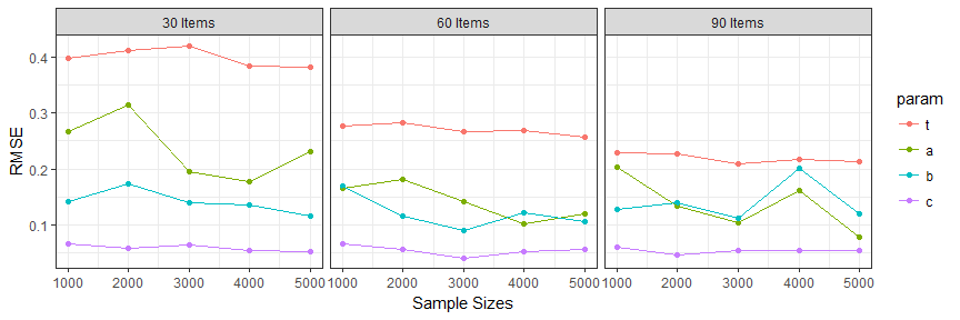

The effects of fixed items on estimation (3000 people and 50 items)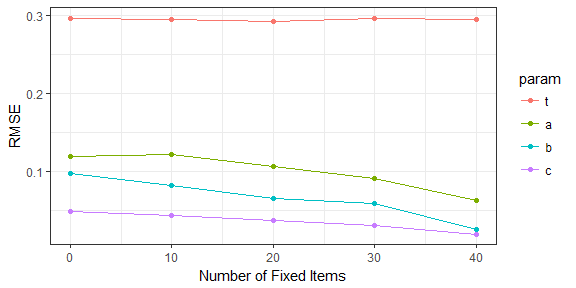

The effect of missing data on estimation (3000 people and 50 items)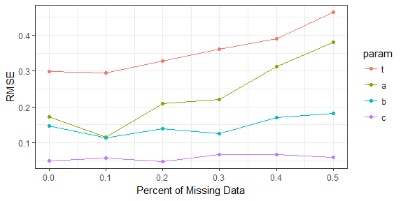

Automated Test Assembly

Automated test assembly (ATA) applies advanced optimization algorithms to assemble test forms that optimize the objective functions while satisfying a set of constraints. Objectives in ATA can be relative (e.g., maximize or minimize difficulty) or absolute (e.g., approach a TIF target). While there are many ATA methods in psychometric literature [5][6][7], the mixed integer linear programming (MILP) algorithm is chosen as the implementation method in this package for its versality and flexibility. This module uses the open source solver lp_solve and the package lpSolveAPI.

The following ATA functions are available:

ata(pool, num_form, len, max_use, group, ...): Create an ATA job. Use len and max_use to conveniently set test length constraint and the maximum item usage constraint. Use group (a string to refer to a variable in the item pool or a numeric vector of group coding) to group item belonging to the same sets.
ata_obj_relative(x, coef, mode, negative, flatten, forms, collapse): Add a relative objective function to the ATA job. Use mode to indicate whether to maximize (mode="max") or minimize (mode="min") the objective functions. coef is the coefficients in the objective functions, which can be a variable of the item pool or a pool-long numeric vector. When being a numeric vector unequal to the number of items in the pool, it is interpreted as θ points at which the information is optimized. Use negative=TRUE to indicate that the value of the objective function is expected to be negative. Use forms to indicate onto which forms objective functions are set (NULL for all forms). Use collapse=TRUE to collapse objective functions on different forms into one objective function. Tune the flatten argument if a flat TIF is desired.
ata_obj_absolute(x, coef, target, forms, collapse): Add an absolute objective function to the ATA job. Use target to set the target values.
ata_constraint(x, coef, min, max, level, forms, collapse): Add a constraint to the ATA job. coef can be either a variable of the item pool, a pool-long numeric vector, or a single value (broadcasted to all items). When coef refers to a categorical variable, use level to indicate for which level the constraint is set. When coef refers to a quantitative variable, leave level=NULL.
ata_item_use(x, min, max, items): Set the minimum and maximum usage constraints on items. items should be a vector of item indices in the pool.
ata_item_enemy(x, items): Set the enemy relationship constraints on items.
ata_item_fixedvalue(x, items, min, max, forms, collapse): Fix the results of decision variables on items
ata_solve(x, as.list, timeout, ...): Solve the ATA job. Use as.list=TRUE to return results as list; otherwise, data frame. Use timeout to set the time limits of the job in seconds. Pass additional control parameters in .... See the documentation of lp_solve and lpSolveAPI for more details. Once solved, the ATA job is added with four objects: status (status code of the solution), optimum (final optimal value of the objective function), result (a binary matrix of assembly results), and item (a list of data frame of assembled test forms).
plot.ata(x, ...): Plot the TIFs of assembled test forms.

Examples

Generate a pool of 300 items

pool <- with(model_3pl_gendata(1, 300), data.frame(a=a, b=b, c=c))
pool$id <- 1:nrow(pool)
pool$content <- sample(1:3, nrow(pool), replace=TRUE)
pool$time <- round(rlnorm(nrow(pool), 4.2, .3))
pool$group <- sort(sample(1:round(nrow(pool)/3), nrow(pool), replace=TRUE))

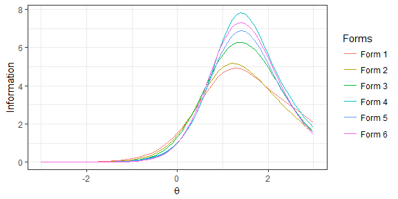
Ex. 1: 6 forms, 10 items, maximize b parameter

x <- ata(pool, 6, len=10, max_use=1)
x <- ata_obj_relative(x, "b", "max")
x <- ata_solve(x)
plot(x)

sapply(x$items, function(x) c(n=nrow(x), b_mean=mean(x$b), b_sd=sd(x$b))) %>% t()

##       n   b_mean      b_sd
## [1,] 10 1.420730 0.6934977
## [2,] 10 1.432549 0.4756749
## [3,] 10 1.409530 0.3642590
## [4,] 10 1.427461 0.4112808
## [5,] 10 1.407538 0.4923109
## [6,] 10 1.398415 0.2282698

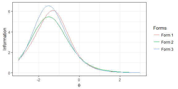
Ex. 2: 3 forms, 10 items, minimize b parameter

x <- ata(pool, 3, len=10, max_use=1)
x <- ata_obj_relative(x, "b", "min", negative=TRUE)
x <- ata_solve(x, as.list=FALSE, timeout=5)
plot(x)

group_by(x$items, form) %>% summarise(n=n(), b_mean=mean(b), b_sd=sd(b))

## # A tibble: 3 x 4
##    form     n b_mean  b_sd
##   <int> <int>  <dbl> <dbl>
## 1     1    10  -1.62 0.445
## 2     2    10  -1.62 0.349
## 3     3    10  -1.61 0.291

Ex. 3: 2 forms, 10 items, mean(b) = 0, sd(b) = 1.0, content = (3, 3, 4)

x <- ata(pool, 2, len=10, max_use=1)
x <- ata_obj_absolute(x, pool$b, 0 * 10)
x <- ata_obj_absolute(x, (pool$b - 0)^2, 1 * 10)
x <- ata_constraint(x, "content", min=3, max=3, level=1)
x <- ata_constraint(x, "content", min=3, max=3, level=2)
x <- ata_constraint(x, "content", min=4, max=4, level=3)
x <- ata_solve(x, timeout=5)
plot(x)

sapply(x$items, function(x) c(n=nrow(x), b_mean=mean(x$b), b_sd=sd(x$b))) %>% t()

##       n      b_mean     b_sd
## [1,] 10 0.002175360 1.053551
## [2,] 10 0.007400645 1.050613

Ex. 4: Same with ex. 3, but group-based

x <- ata(pool, 2, len=10, max_use=1, group="group")
x <- ata_obj_absolute(x, pool$b, 0 * 10)
x <- ata_obj_absolute(x, (pool$b - 0)^2, 1 * 10)
x <- ata_constraint(x, "content", min=3, max=3, level=1)
x <- ata_constraint(x, "content", min=3, max=3, level=2)
x <- ata_constraint(x, "content", min=4, max=4, level=3)
x <- ata_solve(x, as.list=FALSE, timeout=10)
plot(x)

group_by(x$items, form) %>% summarise(n=n(), b_mean=mean(b), b_sd=sd(b), n_items=length(unique(id)), n_groups=length(unique(group)))

## # A tibble: 2 x 6
##    form     n    b_mean  b_sd n_items n_groups
##   <int> <int>     <dbl> <dbl>   <int>    <int>
## 1     1    10 -0.00898   1.03      10        6
## 2     2    10 -0.000522  1.05      10        6

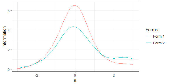
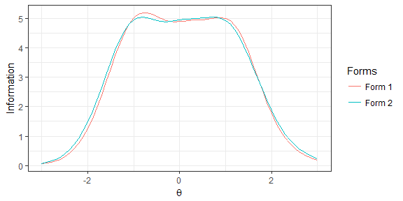
Ex. 5: 2 forms, 10 items, flat TIF over [-1, 1]

x <- ata(pool, 2, len=10, max_use=1)
x <- ata_obj_relative(x, seq(-1, 1, by=.5), "max")
x <- ata_solve(x)

## the model is sub-optimal, optimum: 4.848 (4.942, 0.094)

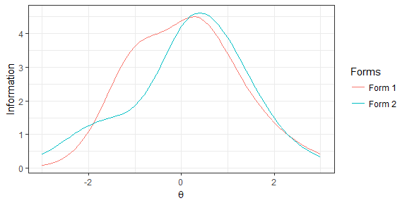
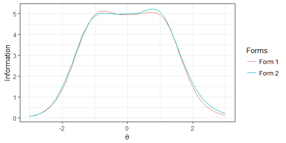
plot(x)

Ex. 6: 2 forms, 10 items, info target over [-1, 1] to be 5.0

x <- ata(pool, 2, len=10, max_use=1)
x <- ata_obj_absolute(x, seq(-1, 1, by=.5), 5.0)
x <- ata_solve(x, timeout=10)
plot(x)

Computerized Adaptive Testing

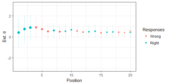
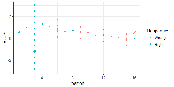
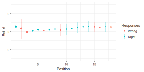
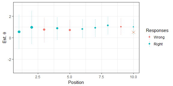
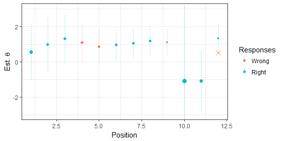
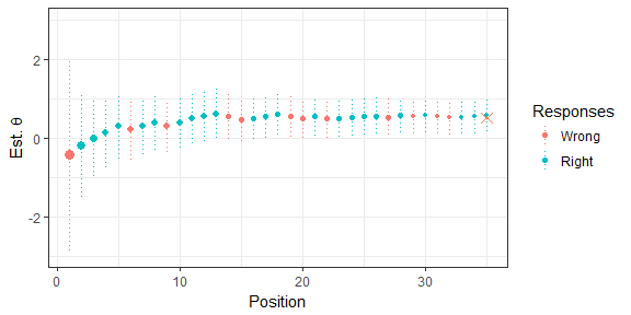
Computerized adaptive testing (CAT) is a testing model that utilizes the computing powers of modern computers to customize the test form on-the-fly to match a test taker's demonstrated abilities. The on-the-fly test adaptation improves testing efficiency and prevents answer-copying behaviors to a great extent. This module provides a framework for conducting CAT simulation studies. Three essential components of a CAT system are: the item selection rule, the ability estimation rule, and the test stopping rule. The framework allows for the mix-and-match of different rules and using customized rules in the CAT simulation. When writing a new rule, the function signature must be function(len, theta, stats, admin, pool, opts) where len is the current test length, theta is the current θ estimate, stats is a matrix of four columns (u, t, se, info), admin is a data frame of administered items, pool is a data frame of remaining items in the pool, opts is a list of option/control parameters (see built-in rules for examples).

The following functions are available in this module:

cat_sim(true, pool, ...): Start a CAT simulation. Pass options into ..., where min (the minimum test length) and max (the maximum test length) are required. Use theta to set the initial value of θ estimate.
cat_estimate_mle: The maximum likelihood estimation rule. Use map_len (10 by default) to apply MAP to the first K items and use map_prior (c(0, 1) by default) to set the prior for MAP. MAP is used to prevent extreme result of MLE.
cat_estimate_eap: The EAP estimation rule. Use eap_mean and eap_sd options to control the prior.
cat_estimate_hybrid: A hybrid estimation rule of MLE (for mixed responses) and EAP (for all 1s or 0s response)
cat_select_maxinfo: The maximum information selection rule[8]. Use group (variable name) to group items belonging to the set. Use info_random to add the random-esque item exposure control.
cat_select_ccat: The constrained CAT selection rule[9]. This rule selects items under the content-balancing constraint. Use ccat_var to indicate the content variable in the pool and use ccat_perc to set the desired content distribution (a vector in which the element name is the content code and the value is the percentage). Use ccat_random to add randomness to initial item selections. Use info_random to add the randomesque item exposure control.
cat_select_shadow: The shadow-test selection rule[10]. Use shadow_id to group item sets. Use constraints to set constraints. Constraints should be in a data frame with four columns: var (variable name), level (variable level, NA for quantitative variable), min (lower bound), and max (upper bound).
cat_stop_default: A three-way stopping rule. When stop_se is set in options, the standard error stopping rule is invoked. When stop_mi is set in options, the minimum information stopping rule is invoked. When stop_cut is set in options, the confidence interval stopping rule is invoked. The width of the confidence interval is controlled by the ci_width option.
cat_stop_projection: The projection-based stopping rule[11]. Use projection_method to choose the projection method (info or diff). Use stop_cut to set the cut score. Use constraints to set the constraints. Constraints should be in a data frame with four columns: var (variable name), level (variable level, NA for quantitative variable), min (lower bound), max (upper bound).
plot.cat(x, ...): Plot the results of a CAT simulation.

Examples

Generate a 100-item pool

num_items <- 100
pool <- with(model_3pl_gendata(1, num_items), data.frame(a=a, b=b, c=c))
pool$group <- sort(sample(1:30, num_items, replace=TRUE))
pool$content <- sample(1:3, num_items, replace=TRUE)
pool$time <- round(rlnorm(num_items, mean=4.1, sd=.2))

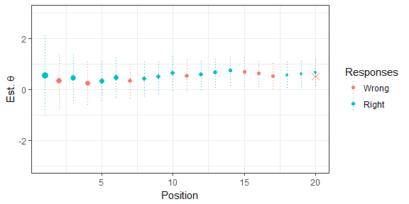
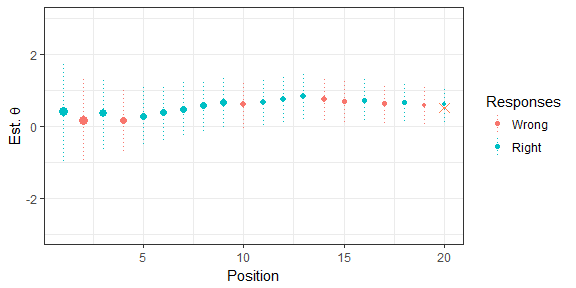
MLE, EAP, and hybrid estimation rule

cat_sim(.5, pool, min=10, max=20, estimate_rule=cat_estimate_mle) %>% plot()

cat_sim(.5, pool, min=10, max=20, estimate_rule=cat_estimate_eap) %>% plot()

cat_sim(.5, pool, min=10, max=20, estimate_rule=cat_estimate_hybrid) %>% plot()

SE, MI, and CI stopping rule

cat_sim(.5, pool, min=10, max=20, stop_se=.3) %>% plot()

cat_sim(.5, pool, min=10, max=20, stop_mi=.6) %>% plot()

cat_sim(.5, pool, min=10, max=20, stop_cut=0) %>% plot()

cat_sim(.5, pool, min=10, max=20, stop_cut=0, ci_width=2.58) %>% plot()

Maximum information selection with item sets

cat_sim(.5, pool, min=10, max=10, group="group")$admin %>% round(., 2)

##    u    t   se info    a     b    c group content time
## 9  1 0.63 0.64 2.48 1.22  0.39 0.12     4       1   46
## 10 0 0.63 0.64 2.48 0.72  0.99 0.07     4       3   59
## 11 1 0.63 0.64 2.48 2.00  0.13 0.11     4       2   46
## 12 1 0.63 0.64 2.48 1.36 -1.43 0.03     4       3   54
## 3  1 0.79 0.48 4.39 1.35  0.71 0.05     2       3   50
## 4  1 0.79 0.48 4.39 1.16 -0.60 0.05     2       3   57
## 5  0 0.79 0.48 4.39 1.03  0.73 0.07     2       2   36
## 6  1 0.79 0.48 4.39 0.79  0.19 0.15     2       1   70
## 80 0 0.71 0.43 5.51 1.07  0.23 0.10    25       1   57
## 81 1 0.71 0.43 5.51 1.04 -0.53 0.06    25       1   65

Maximum information with item exposure control

cat_sim(.5, pool, min=10, max=10, info_random=5)$admin %>% round(., 2)

##    u    t   se info    a     b    c group content time
## 13 1 0.42 1.09 0.85 1.47 -0.14 0.12     5       2   41
## 11 1 0.66 0.75 1.77 2.00  0.13 0.11     4       2   46
## 3  1 1.00 0.73 1.87 1.35  0.71 0.05     2       3   50
## 43 0 0.68 0.52 3.74 1.10  0.55 0.03    15       1   54
## 90 0 0.51 0.44 5.05 1.09  0.64 0.10    28       2   81
## 74 0 0.30 0.40 6.34 1.19  0.01 0.08    23       2   94
## 75 1 0.42 0.38 7.04 1.21  0.36 0.04    23       3   51
## 28 1 0.48 0.36 7.55 1.27 -0.01 0.17    10       1   66
## 48 1 0.53 0.35 8.01 1.25 -0.09 0.08    16       3   63
## 62 1 0.66 0.36 7.83 1.09  0.19 0.09    19       1   48

Constrained-CAT selection rule with and without initial randomness

cat_sim(.5, pool, min=10, max=20, select_rule=cat_select_ccat, ccat_var="content", ccat_perc=c("1"=.2, "2"=.3, "3"=.5))$admin$content %>% freq()

##   value freq perc cum.freq cum.perc
## 1     1    4  0.2        4      0.2
## 2     2    6  0.3       10      0.5
## 3     3   10  0.5       20      1.0

Shadow-test selection rule

cons <- data.frame(var='content', level=1:3, min=c(3,3,4), max=c(3,3,4))
cons <- rbind(cons, data.frame(var='time', level=NA, min=55*10, max=65*10))
cat_sim(.5, pool, min=10, max=10, select_rule=cat_select_shadow, constraints=cons)$admin %>% round(., 2)

##    u    t   se info    a     b    c group content time shadow_id
## 11 1 0.56 0.81 1.53 2.00  0.13 0.11     4       2   46        11
## 3  1 0.95 0.77 1.69 1.35  0.71 0.05     2       3   50         3
## 21 0 0.73 0.59 2.89 1.35  1.16 0.13     8       2   50        21
## 83 0 0.48 0.49 4.13 1.26  0.50 0.13    25       2   65        83
## 75 0 0.31 0.44 5.14 1.21  0.36 0.04    23       3   51        75
## 48 1 0.39 0.41 5.97 1.25 -0.09 0.08    16       3   63        48
## 9  0 0.26 0.38 6.77 1.22  0.39 0.12     4       1   46         9
## 34 0 0.10 0.37 7.15 1.23 -0.08 0.10    13       3   73        34
## 28 1 0.17 0.35 8.27 1.27 -0.01 0.17    10       1   66        28
## 62 0 0.09 0.34 8.66 1.09  0.19 0.09    19       1   48        62

Projection-based stopping rule

cons <- data.frame(var='content', level=1:3, min=5, max=15)
cons <- rbind(cons, data.frame(var='time', level=NA, min=60*20, max=60*40))
cat_sim(.5, pool, min=20, max=40, select_rule=cat_select_shadow, stop_rule=cat_stop_projection, projection_method="diff", stop_cut=0, constraints=cons) %>% plot()

Multistage Testing

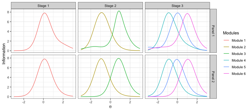
Multistage testing (MST) is a computer-based adaptive testing model that gives practitioners more controls over the test, compared to CAT. MST navigates test takers through multiple stages and each stage contains a set of pre-constructed modules. The test is adapted between stages in order to administer modules most suited to the test taker's ability. A group of modules connected via the routing rule constitutes a MST panel, and the combination of modules (one module per stage) that leads a test taker to the end of the test is called a route. The design, or configuration, of a MST is normally abbreviated as "1-2", "1-3-3", etc., where the length represents the number of stages and each number represents the number of modules in that stage. With reduced adaptivity, MST usually has a slightly low efficiency than CAT. However, it allows test developers to add complex constraints and review assembled tests before publishing and administration, which enhances test quality and security.

The following functions are available in this module:

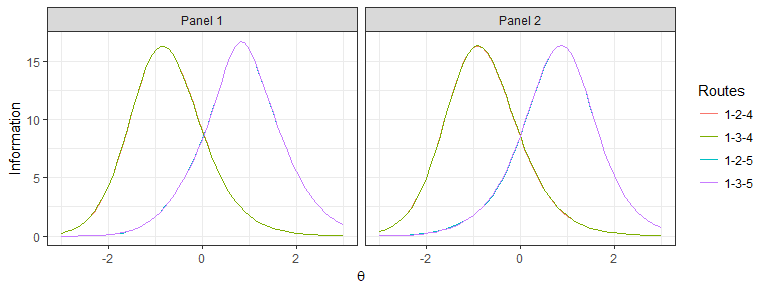
mst(pool, design, num_panel, method, len, max_use, group, ...): Create a MST assembly job. Use design to specify the design/configuration of the MST (e.g., "1-3", "1-2-2", "1-2-3"). Use num_panel to simultaneously assembly multiple panels. method can be either topdown[12] or bottomup[13]. Use len and max_use to conveniently set the test length and maximum item usage. Use group to group item sets.
mst_route(x, route, op): Add or remove a route from the MST
mst_obj(x, theta, indices, target, flatten): Add objective functions to the assembly job. Use theta to specify at which θ points the information is optimized. When target is NULL, the information is maximized at θ points; otherwise, the information approaches the given targets. Use flatten argument to obtain a flatter TIF by curbing the information difference between θ points. indices sets on which modules or routes the objective functions are added.
mst_constraint(x, coef, min, max, level, indices): Add constraints to the assembly job. coef should be a variable name of pool-long numeric vector. Set level=NULL for a quantitative variable and a specific level for a categorical variable.
mst_stage_length(x, stages, min, max): Add the length constraints on modules in given stages.
mst_rdp(x, theta, indices, tol): Set the routing decision points between two adjacent modules.
mst_module_mininfo(x, theta, mininfo, indices): Set the minimum information at given θ points for some modules.
mst_assemble(x, ...): Assemble MST panels.
mst_get_items(x, panel, stage, module, route, route_index): Extract assembled modules.
plot.mst(x, ...): Plot TIFs of assembled routes (when byroute=TRUE) or modules (when byroute=FALSE).
mst_sim(x, true, rdp, ...): Simulate a MST administration. When rdp=NULL, test takers are routed to the module with the maximum information; otherwise test takers are routed according to given routing decision points.

Examples

Generate a pool of 300 items

num_item <- 300
pool <- with(model_3pl_gendata(1, num_item), data.frame(a=a, b=b, c=c))
pool$id <- 1:num_item
pool$content <- sample(1:3, num_item, replace=TRUE)
pool$time <- round(rlnorm(num_item, 4, .3))
pool$group <- sort(sample(1:round(num_item/3), num_item, replace=TRUE))

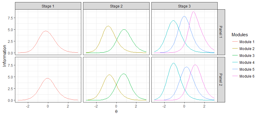
Ex. 1: Assemble 2 panels of 1-2-2 MST using the top-down approach 20 items in total and 10 items in content area 1 in each route maximize info. at -1 and 1 for easy and hard routes

x <- mst(pool, "1-2-2", 2, 'topdown', len=20, max_use=1)
x <- mst_obj(x, theta=-1, indices=1:2)
x <- mst_obj(x, theta=1, indices=3:4)
x <- mst_constraint(x, "content", 10, 10, level=1)
x <- mst_assemble(x, timeout=10)
plot(x, byroute=TRUE)

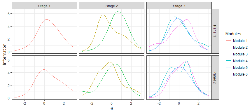
Ex. 2: Assemble 2 panels of 1-2-3 MST using the bottom-up approach Remove two routes with large theta change: 1-2-6, 1-3-4 10 items in total and 4 items in content area 2 in each module Maximize info. at -1, 0 and 1 for easy, medium, and hard modules

x <- mst(pool, "1-2-3", 2, 'bottomup', len=10, max_use=1)
x <- mst_route(x, c(1, 2, 6), "-")
x <- mst_route(x, c(1, 3, 4), "-")
x <- mst_obj(x, theta= 0, indices=c(1, 5))
x <- mst_obj(x, theta=-1, indices=c(2, 4))
x <- mst_obj(x, theta= 1, indices=c(3, 6))
x <- mst_constraint(x, "content", 4, 4, level=2)
x <- mst_assemble(x, timeout=10) 
plot(x, byroute=FALSE)

Ex.3: Same specs with Ex.2 (without content constraints), but group-based

x <- mst(pool, "1-2-3", 2, 'bottomup', len=12, max_use=1, group="group")
x <- mst_route(x, c(1, 2, 6), "-")
x <- mst_route(x, c(1, 3, 4), "-")
x <- mst_obj(x, theta= 0, indices=c(1, 5))
x <- mst_obj(x, theta=-1, indices=c(2, 4))
x <- mst_obj(x, theta= 1, indices=c(3, 6))
x <- mst_assemble(x, timeout=10)
plot(x, byroute=FALSE)

for(p in 1:x$num_panel)
   for(m in 1:x$num_module){
     items <- mst_get_items(x, panel=p, module=m)
     cat('panel=', p, ', module=', m, ': ', length(unique(items$id)), ' items from ', 
         length(unique(items$group)), ' groups\n', sep='')
   }

## panel=1, module=1: 12 items from 3 groups
## panel=1, module=2: 12 items from 6 groups
## panel=1, module=3: 12 items from 4 groups
## panel=1, module=4: 12 items from 6 groups
## panel=1, module=5: 12 items from 4 groups
## panel=1, module=6: 12 items from 5 groups
## panel=2, module=1: 12 items from 4 groups
## panel=2, module=2: 12 items from 6 groups
## panel=2, module=3: 12 items from 3 groups
## panel=2, module=4: 12 items from 4 groups
## panel=2, module=5: 12 items from 4 groups
## panel=2, module=6: 12 items from 4 groups

Ex.4: Assemble 2 panels of 1-2-3 using the top-down design 20 total items and 10 items in content area 3, 6+ items in stage 1 & 2

x <- mst(pool, "1-2-3", 2, "topdown", len=20, max_use=1)
x <- mst_route(x, c(1, 2, 6), "-")
x <- mst_route(x, c(1, 3, 4), "-")
x <- mst_obj(x, theta=-1, indices=1)
x <- mst_obj(x, theta=0, indices=2:3)
x <- mst_obj(x, theta=1, indices=4)
x <- mst_constraint(x, "content", 8, 12, level=3)
x <- mst_stage_length(x, 1:2, min=6)
x <- mst_assemble(x, timeout=15)
plot(x, byroute=FALSE)

for(p in 1:x$num_panel)
  for(s in 1:x$num_stage){
    items <- mst_get_items(x, panel=p, stage=s)
    cat('panel=', p, ', stage=', s, ': ', length(unique(items$id)), ' items\n', sep='')
    }

## panel=1, stage=1: 6 items
## panel=1, stage=2: 12 items
## panel=1, stage=3: 24 items
## panel=2, stage=1: 6 items
## panel=2, stage=2: 12 items
## panel=2, stage=3: 24 items

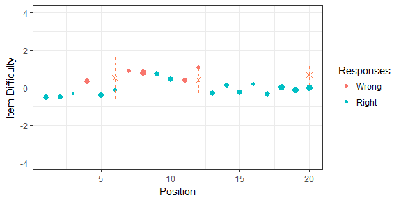
Ex. 5: Administer the MST using fixed RDP for routing

x_sim <- mst_sim(x, .5, list(stage1=0, stage2=c(-.4, .4)))
plot(x_sim, ylim=c(-4, 4))

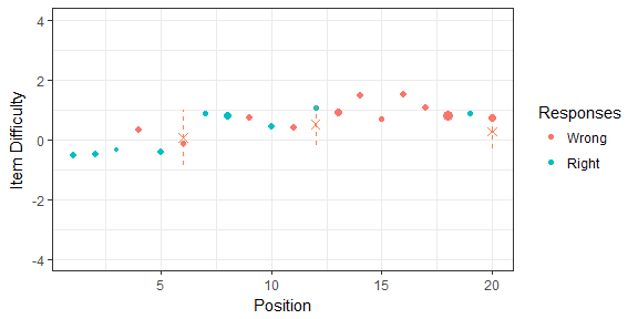
Ex. 6: Administer the MST using the maximum information for routing

x_sim <- mst_sim(x, .5)
plot(x_sim, ylim=c(-4, 4))

Ending

Please send comments, questions and feature requests to the author. To report bugs, go to the issues page.

References

[1] Birnbaum, A. (1968). Some latent trait models. In F.M. Lord & M.R. Novick, (Eds.), Statistical theories of mental test scores. Reading, MA: Addison-Wesley.

[2] Rasch, G. (1966). An item analysis which takes individual differences into account. British journal of mathematical and statistical psychology, 19(1), 49-57.

[3] Muraki, E. (1992). A Generalized Partial Credit Model: Application of an EM Algorithm. Applied Psychological Measurement, 16(2), 159-176.

[4] Muraki, E. (1993). Information Functions of the Generalized Partial Credit Model. Applied Psychological Measurement, 17(4), 351-363.

[5] Stocking, M. L., & Swanson, L. (1998). Optimal design of item banks for computerized adaptive tests. Applied Psychological Measurement, 22, 271-279.

[6] Luecht, R. M. (1998). Computer-assisted test assembly using optimization heuristics. Applied Psychological Measurement, 22, 224-236.

[7] van der Linden, W. J., & Reese, L. M. (1998). A model for optimal constrained adaptive testing. Applied Psychological Measurement, 22, 259-270.

[8] Weiss, D. J., & Kingsbury, G. (1984). Application of computerized adaptive testing to educational problems. Journal of Educational Measurement, 21, 361-375.

[9] Kingsbury, C. G., & Zara, A. R. (1991). A comparison of procedures for content-sensitive item selection in computerized adaptive tests. Applied Measurement in Education, 4, 241-261.

[10] van der Linden, W. J. (2000). Constrained adaptive testing with shadow tests. In Computerized adaptive testing: Theory and practice (pp. 27-52). Springer Netherlands.

[11] Luo, X., Kim, D., & Dickison, P. (2018). Projection-based stopping rules for computerized adaptive testing in licensure testing. Applied Psychological Measurement, 42, 275-290

[12] Luo, X., & Kim, D. (2018). A Top‐Down Approach to Designing the Computerized Adaptive Multistage Test. Journal of Educational Measurement, 55(2), 243-263.

[13] Luecht, R. M., & Nungester, R. J. (1998). Some practical examples of computer‐adaptive sequential testing. Journal of Educational Measurement, 35(3), 229-249.

giadasp/xxIRT

xxIRT: Item Response Theory and Computer-Based Testing in R

Table of Contents

Installation

Introduction

Package Modules

IRT Models

3PL Model

Examples

Graphs

Generalized Partial Credit Model

Examples

Graphs

Parameter Estimation

Examples

Automated Test Assembly

Examples

Computerized Adaptive Testing

Examples

Multistage Testing

Examples

Ending

References