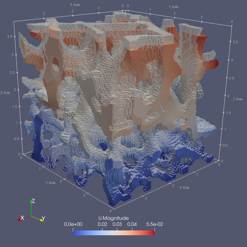
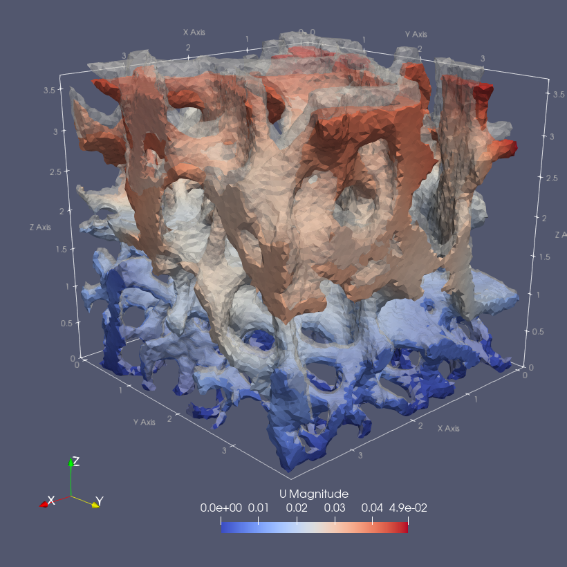
Computed Tomography to Finite Elements.
Micro Finite Element (microFE) models can be derived from micro Computed Tomography (microCT) 3D images to non-destructively assess mechanical properties of biological or artificial specimens.
ciclope provides fully open-source pipelines from microCT data preprocessing to microFE model generation, solution and postprocessing.
For mesh generation, ciclope requires pygalmesh, a Python frontend to CGAL.
Follow the installation procedure for CGAL and Eigen.
After that, install pygalmesh with pip or conda
conda install -c conda-forge pygalmesh
After installing pygalmesh, you can install ciclope using pip. The flag [all] will install optional dependencies needed to run full pipelines and examples.
pip install ciclope[all]
Some examples will require DXchange. You can install it with
conda install -c conda-forge dxchangeTo verify your installation checkout this repository and run the tests with the command
cd test
python -m unittest -v test_ciclope.run_tests
If you want to contribute to this project, please install ciclope following the development guide.
ciclope pipelines can be run from the command line as a script. Scroll down and take a look at the Examples folder for this type of use. To view the command line script help run
ciclope -h
To use ciclope within python, import the package with
import ciclopeciclope.utils contains functions that help you read and pre-process 3D datasets for FE model generation.
Read 3D CT dataset stored as stack of TIFFs
from ciclope.utils.recon_utils import read_tiff_stack

input_file = './test_data/LHDL/3155_D_4_bc/cropped/3155_D_4_bc_0000.tif'

data_3D = read_tiff_stack(input_file)
vs = np.ones(3) * 0.06  # voxelsize [mm]
read_tiff_stack reads all TIFF files (slices) contained in the input_file folder. The volume is stored in a 3D numpy.ndarray with size [slices, rows, columns].
Segment and remove unconnected voxels
from skimage import morphology
from ciclope.utils.preprocess import remove_unconnected

BW = data_3D > 142 # fixed global threshold
BW = morphology.closing(BW, morphology.ball(2)) # optional step
L = remove_unconnected(BW)If you already have a mesh file, you can skip the mesh generation steps and use ciclope with 3D meshio objects.
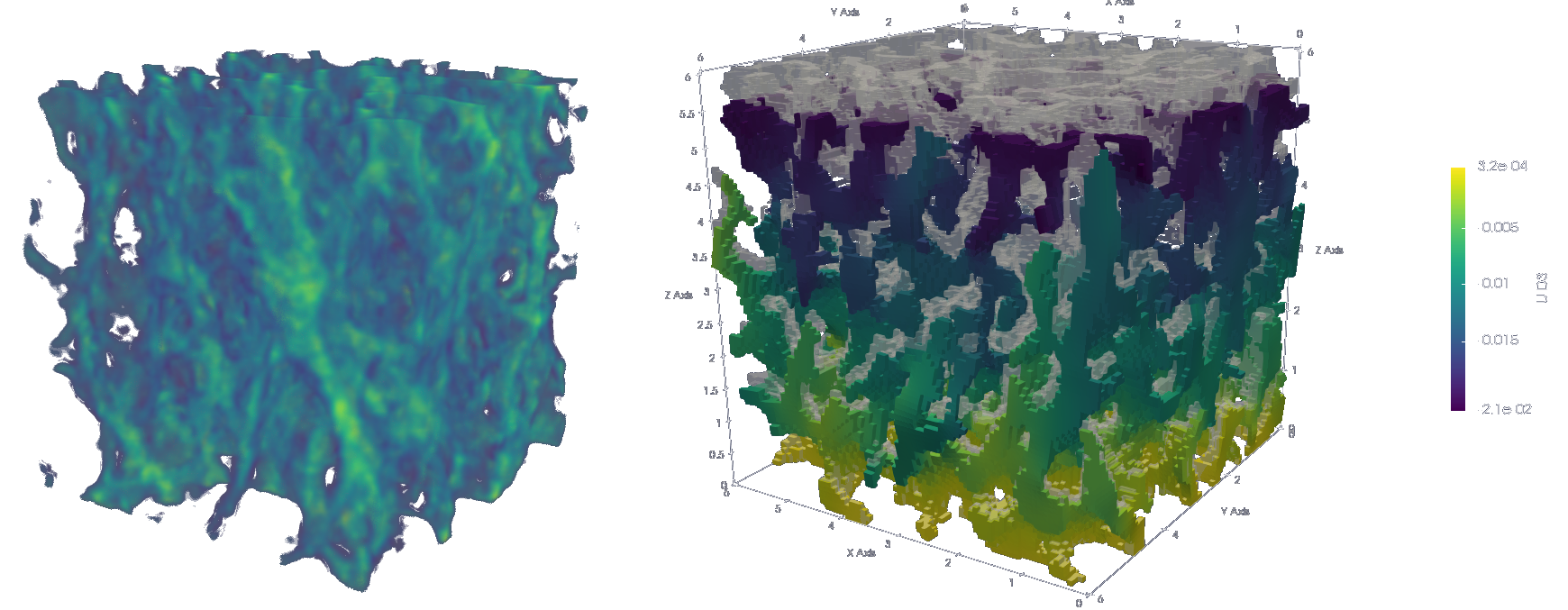 Generate unstructured grid mesh of hexahedra (voxels)
import ciclope
mesh = ciclope.core.voxelFE.vol2ugrid(data_3D, vs)
Generate CalculiX input file .INP for voxel-FE model of linear elastic compression test
input_template = "./input_templates/tmp_example01_comp_static_bone.inp"
ciclope.core.voxelFE.mesh2voxelfe(mesh, input_template, 'foo.inp', keywords=['NSET', 'ELSET'])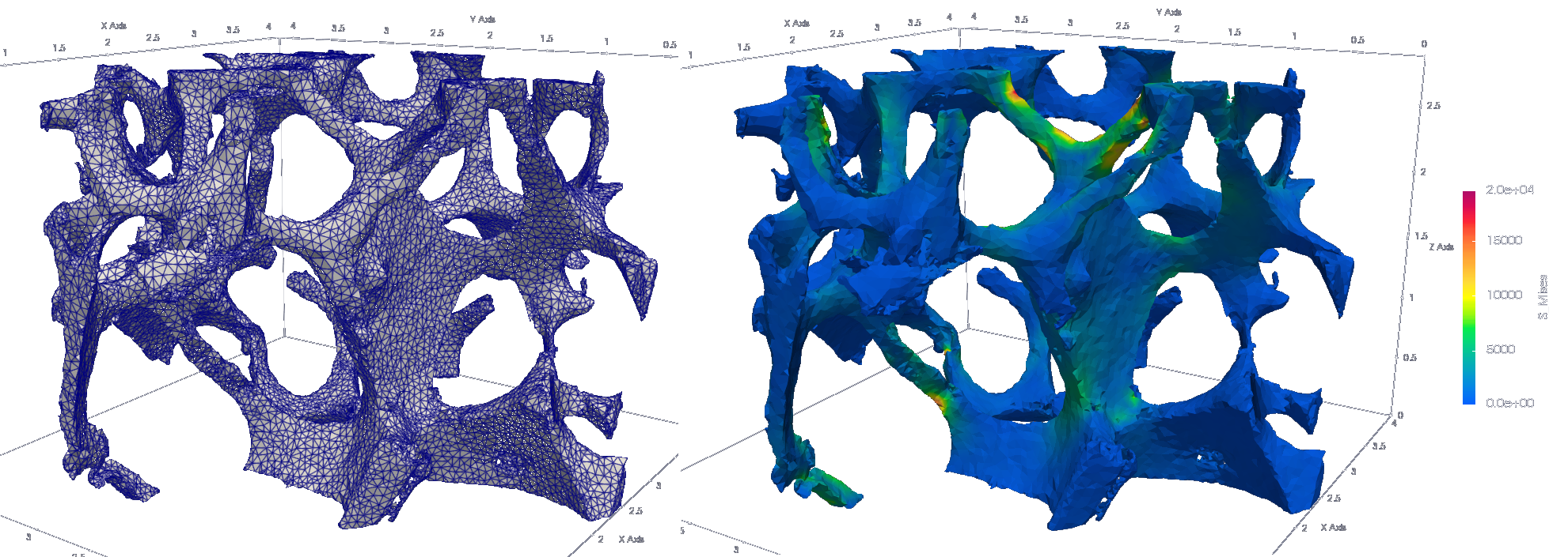 Generate mesh of tetrahedra.
 ciclope uses pygalmesh for tetrahedra mesh generation
mesh = ciclope.core.tetraFE.cgal_mesh(L, vs, 'tetra', max_facet_distance=0.2, max_cell_circumradius=0.1)Generate CalculiX input file .INP for tetrahedra-FE model of non-linear tensile test
input_template = "./input_templates/tmp_example02_tens_static_steel.inp"
ciclope.core.tetraFE.mesh2tetrafe(mesh, input_template, 'foo.inp', keywords=['NSET', 'ELSET'])ciclope.utils.postprocess.paraviewplot calls ParaView to generate and save plots of a chosen model scalar field.
- Add path to your ParaView installation with
import sys
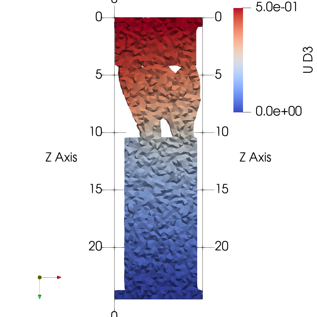
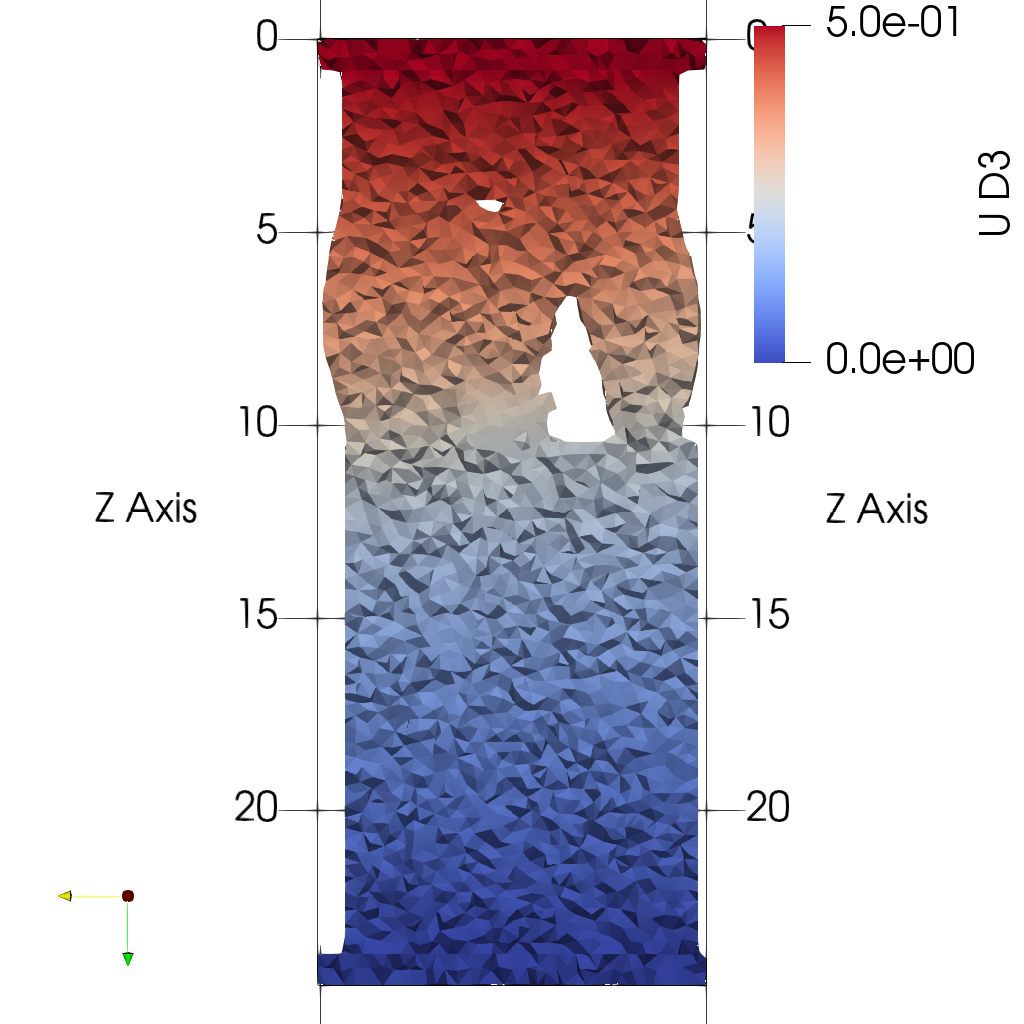
sys.path.append('~/Applications/ParaView-5.9.0-RC1-MPI-Linux-Python3.8-64bit/lib/python3.8/site-packages')- Plot midplanes of the vertical displacement field
UD3
ciclope.utils.postprocess.paraview_plot('test_data/tooth/results/Tooth_3_scaled_2.vtk', slicenormal="xyz",
                                        RepresentationType="Surface", Crinkle=True, ColorBy=['U', 'D2'], Roll=90,
                                        ImageResolution=[1024, 1024], TransparentBackground=True,
colormap='Cool to Warm')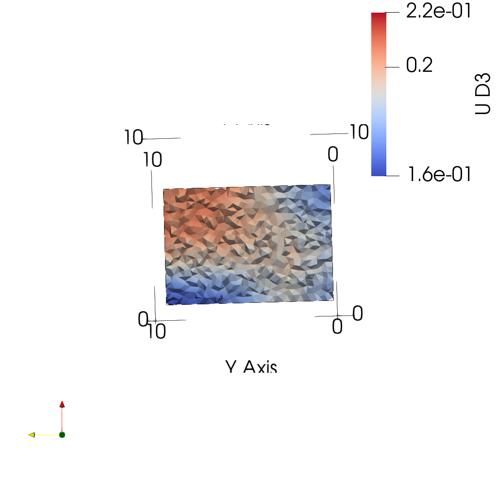 |
 |
 |
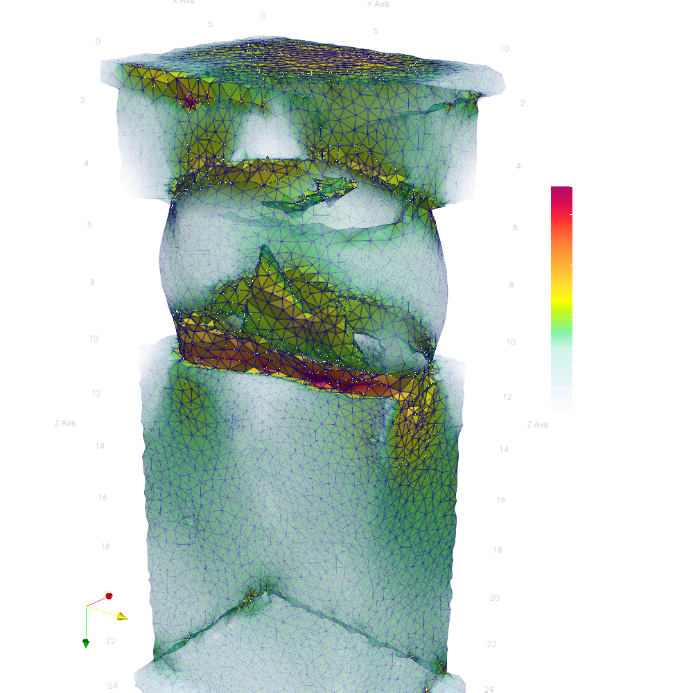
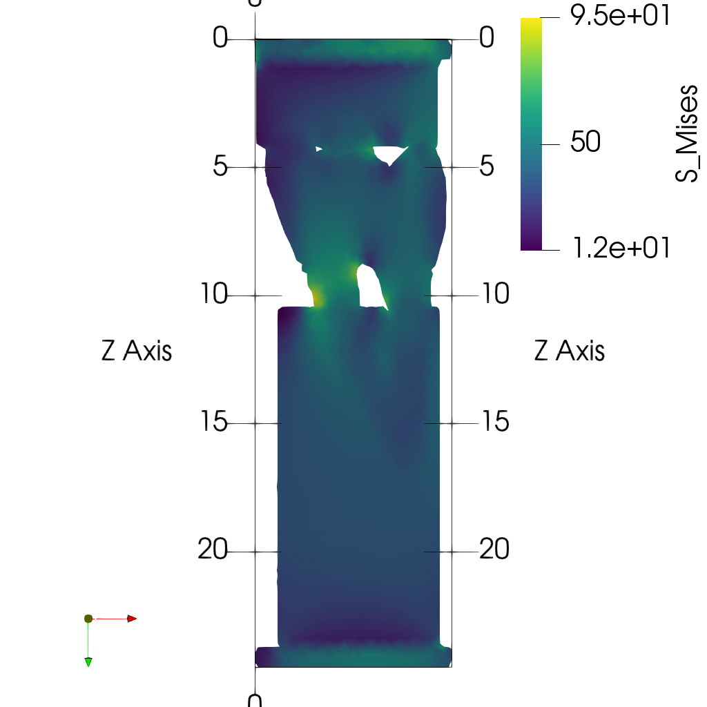
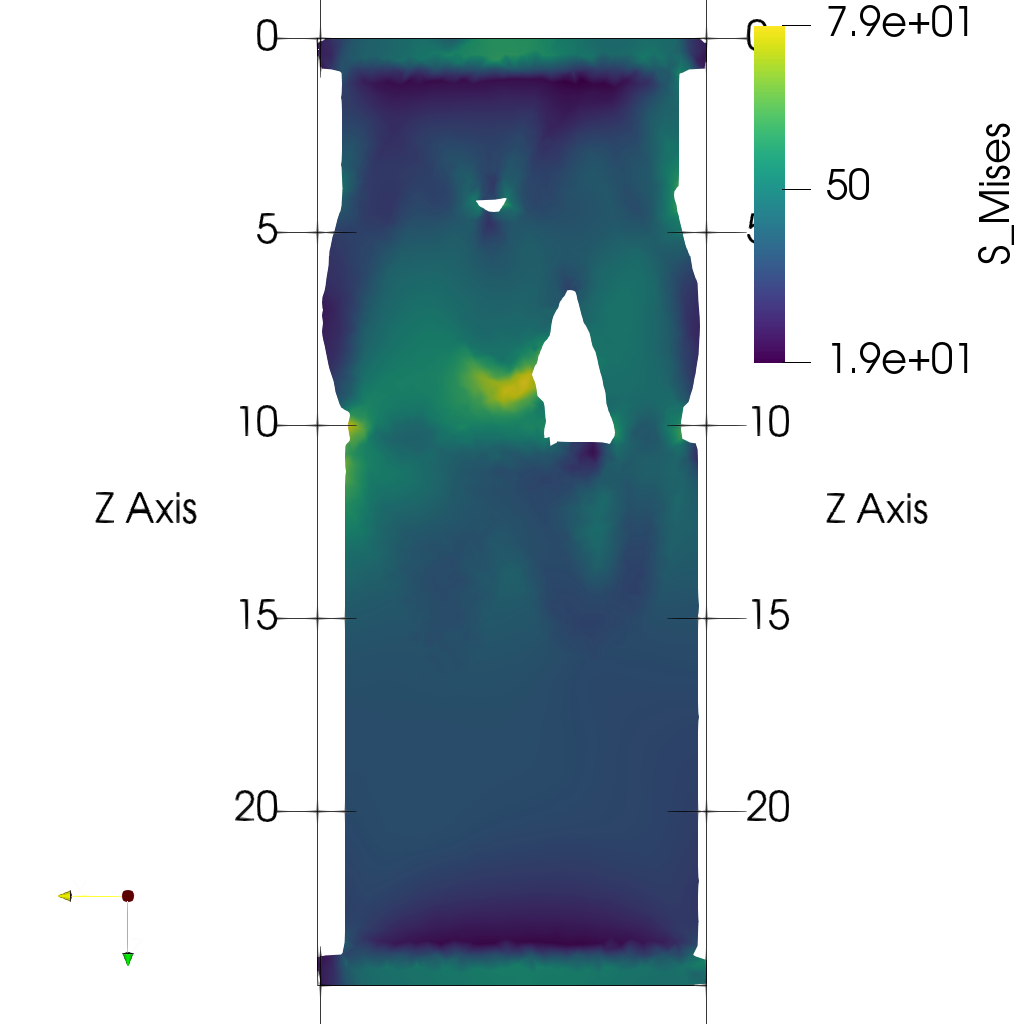
- Plot midplanes of the Von Mises stress
S_Mises
ciclope.utils.postprocess.paraview_plot("test_data/tooth/results/Tooth_3_scaled_2.vtk", slicenormal="xyz",
                                        RepresentationType="Surface", Crinkle=False, ColorBy="S_Mises", Roll=90,
ImageResolution=[1024, 1024])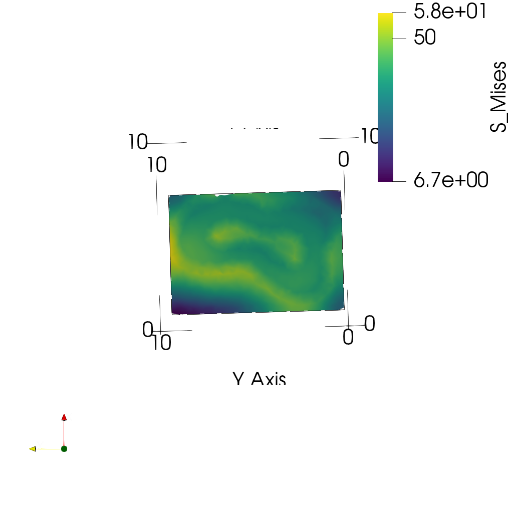 |
 |
 |
See the Jupyter Notebooks in the examples section for more examples of 3D data and results visualization.
The following table shows a general pipeline for FE model generation from CT data that can be executed from the command line with the ciclope script:
| # | Step | Description | command line script flag |
|---|---|---|---|
| 1. | Load CT data | ||
| 2. | Pre-processing | Gaussian smooth | --smooth |
| Resize image | -r |
||
| Add embedding | (not implemented yet) | ||
| Add caps | --caps |
||
| 3. | Segmentation | Uses Otsu method if left empty | -t |
| Remove unconnected voxels | |||
| 4. | Meshing | Outer shell mesh of triangles | --shell_mesh |
| Volume mesh of tetrahedra | --vol_mesh |
||
| 5. | FE model generation | Apply Boundary Conditions | |
| Material mapping | -m, --mapping |
||
| Voxel FE | --voxelfe |
||
| Tetrahedra FE | --tetrafe |
- Tetrahedra meshes are generated with pygalmesh (a Python frontend to CGAL)
- High-resolution surface meshes for visualization are generated with the PyMCubes module.
- All mesh exports are performed with the meshio module.
- ciclope handles the definition of material properties and FE analysis parameters (e.g. boundary conditions, simulation steps..) through separate template files. The folders material_properties and input_templates contain a library of template files that can be used to generate FE simulations.
The pipeline can be executed from the command line with:
ciclope test_data/LHDL/3155_D_4_bc/cropped/3155_D_4_bc_0000.tif test_data/LHDL/3155_D_4_bc/results/3155_D_4_bc_voxelFE.inp -vs 0.0195 0.0195 0.0195 -r 2 -t 63 --smooth 1 --voxelfe --template input_templates/tmp_example01_comp_static_bone.inp --verbose
The example shows how to:
- Load and inspect microCT volume data
- Apply Gaussian smooth
- Resample the dataset
- Segment the bone tissue
- Remove unconnected clusters of voxels
- Convert the 3D binary to a voxel-FE model for simulation in CalculX or Abaqus
- Linear, static analysis; displacement-driven
- Local material mapping (dataset Grey Values to bone Tissue Elastic Modulus)
- Launch simulation in Calculix
- Convert Calculix output to .VTK for visualization in Paraview
- Visualize simulation results in Paraview
The pipeline can be executed from the command line with:
ciclope test_data/LHDL/3155_D_4_bc/cropped/3155_D_4_bc_0000.tif test_data/LHDL/3155_D_4_bc/results/3155_D_4_bc.inp -vs 0.0195 0.0195 0.0195 -r 2 -t 63 --smooth 1 --tetrafe --max_facet_distance 0.025 --max_cell_circumradius 0.05 --vol_mesh --template input_templates/tmp_example01_comp_static_bone.inp
The pipeline can be executed from the command line with:
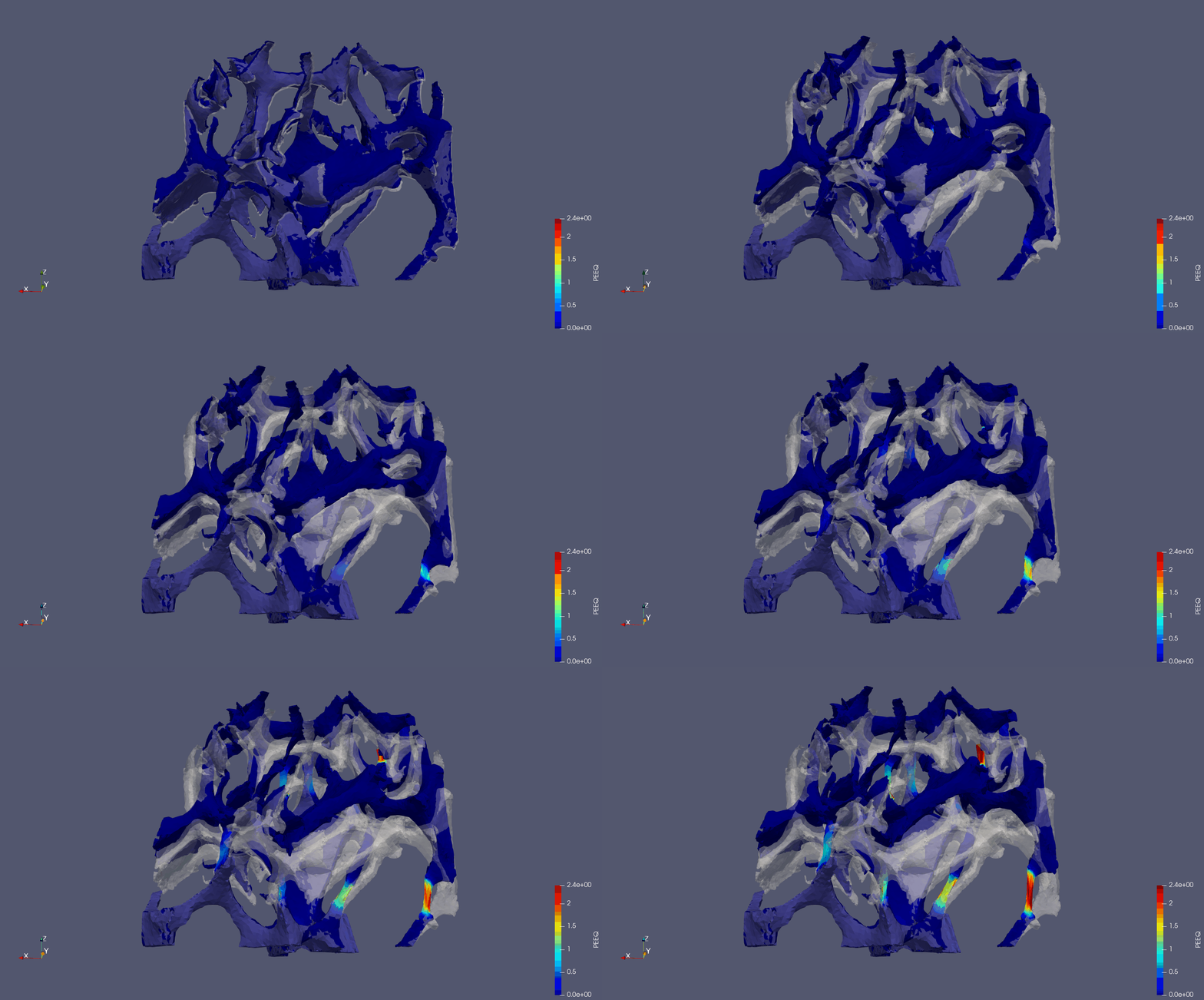
ciclope input.tif output.inp -vs 0.0065 0.0065 0.0065 --smooth -r 1.2 -t 90 --vol_mesh --tetrafe --template ./../input_templates/tmp_example02_tens_Nlgeom_steel.inp -v
The example shows how to:
- Load and inspect synchrotron microCT volume data
- Apply Gaussian smooth
- Resample the dataset
- Segment the steel
- Remove unconnected clusters of voxels
- Generate volume mesh of tetrahedra
- Generate high-resolution mesh of triangles of the model outer shell (for visualization)
- Convert the 3D binary to a tetrahedra-FE model for simulation in CalculX or Abaqus
- Non-linear, quasi-static analysis definition: tensile test with material plasticity. For more info visit: github.com/mkraska/CalculiX-Examples
- Local material mapping
- Launch simulation in Calculix
- Convert Calculix output to .VTK for visualization in Paraview
- Visualize simulation results in Paraview
This project was partially developed during the Jupyter Community Workshop “Building the Jupyter Community in Musculoskeletal Imaging Research” sponsored by NUMFocus.


