Linux pulsar software for recording and analysis

A step by step guide to receive for the first time the B0329+54 pulsar

package produced by Giorgio Dell'Immagine and Andrea Dell‘Immagine, IW5BHY
Summary by Hannes Fasching, OE5JFL oe5jfl(at)aon.at

Installation of the distribution
First boot setup
Supported SDRs
Testing out the SDR dongle
Recording
Conversion
Setting up Tempo
Analysis

Installation of the distribution

First of all get the link for downloading the ISO file (2GB) from Andrea or me (OE5JFL)
make a bootable USB stick using any tool that permit it, dd if you are on linux or rufus if you are on windows; here's an example configuration of rufus:
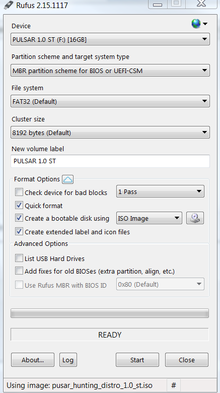
once the process is finished you should see these files on the stick:
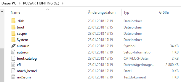
boot from the stick you have flashed changing the boot priority in the BIOS of your system (for most of modern PCs this is done automatically)
once the bootloader (grub) shows up select the first option (run linux)
if you want to install the OS onto your PC run ubiquity tool by double-clicking the install icon on the Desktop
proceed with normal installation of Ubuntu OS (it should be easy but if you're struggling with it you can find tons of guides online like this one)

If you don't want to install the OS on your computer you can continue using the system without running the ubiquity installer (this is called live mode); keep in mind however that all the files that are not witten on an physical HD (e.g. your PC's HD) will be lost when you shutdown the system!

First boot setup

After the first boot, open the terminal and the initialization will start; some links will be created on the Desktop.
Then if you want to optimize the performace of FFT calculations you can run

presto-makewisdom

Keep in mind that this is a long test that can reqire 20-30 min to complete.

Supported SDRs

RTL-SDR up to 2.4 MSps
Airspy up to 10 MSps
Hack-RF up to 20 MSps

Testing out the SDR dongle

To test out the dongle you can run in the terminal

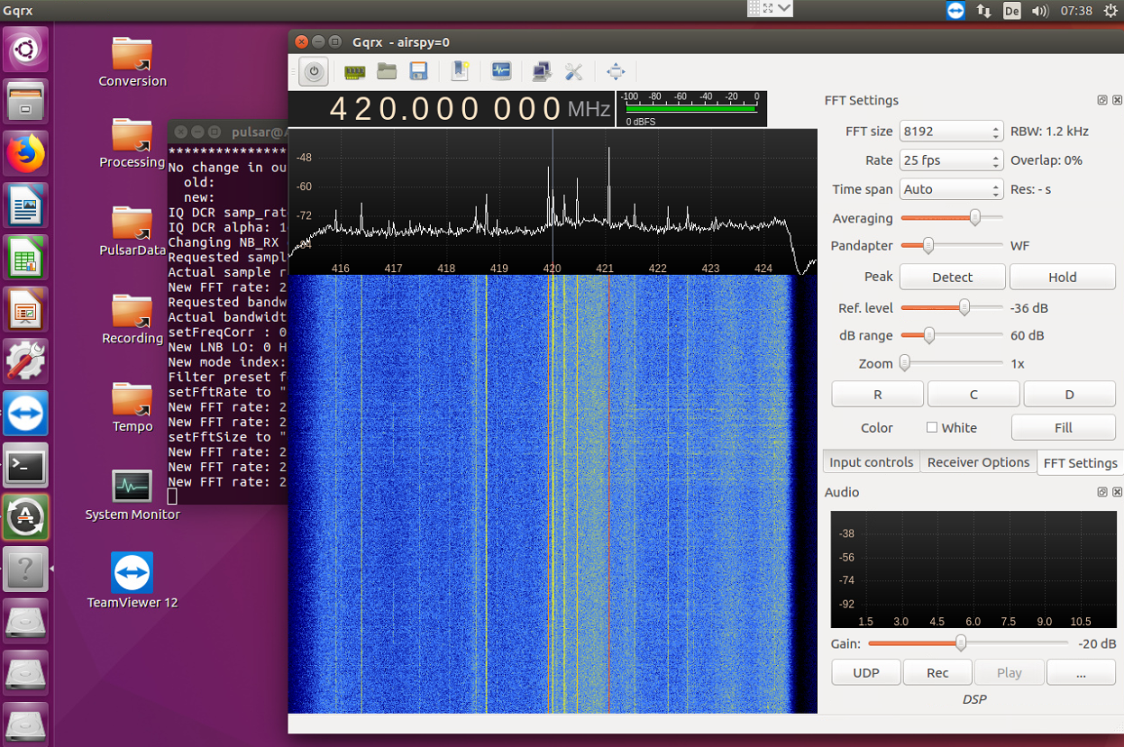
gqrx

after starting you should see the waterfall.
This is a basic SDR interface that should be fine if you want to test and experiment with gain, bandwidth and clearness of the band.

To make sure that your PC can handle the realtime acquisition you can do these tests:

make sure that in the terminal don't appears O characthers. These means 'overflow', so a loss of data that is not tolerable during recording.
open the System Monitor (icon on Desktop) and look at the CPU usage: this should be < 80% while gqrx is running

Recording

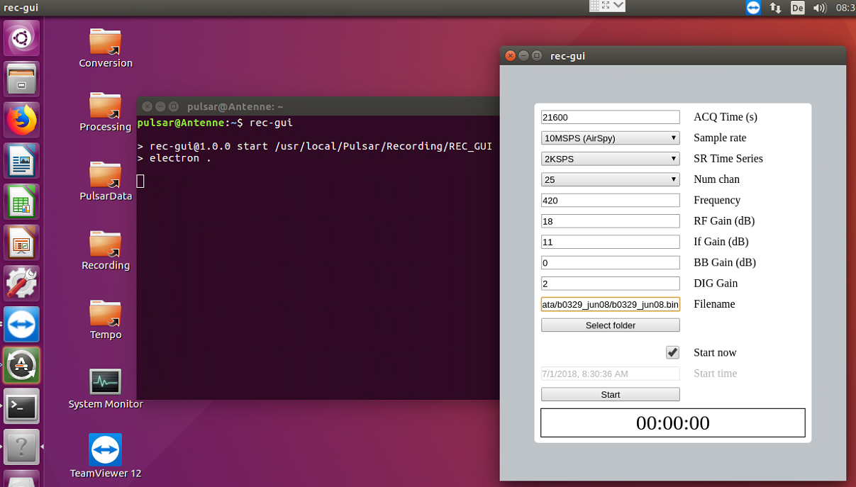
For recording data from the dongle there is a graphical program. To start type in the terminal

rec-gui

and wait the tool to start.

ACQ Time (s) - length of acquisition in seconds
Sample rate - sample rate with the model of SDR dongle
SR Time series - sample rate of the time series (2KSPS is fine for B0329+54)
Num chan - number of channels (25 is fine for B0329+54)
Frequency - center frequency of the acquisition
RF gain - gain of the RF stage of the dongle (supported by all the dongles)
IF gain - gain of the intermediate frequency stage of the dongle (supported by Airspy and HackRf only)
BB gain - gain of the base band stage of the dongle (supported by HackRf only)
DIG gain - software digital gain (2 is fine for most cases)
Filename - file name to write on (you can select the folder first then change the name of the file)

Keep in mind that PulsarData folder on Desktop is supposed to contain the acquisitions files, however you can place them wherever you want

Start now / Start time - you can choose to start now the recording or set a date/time scheudle

To change default values for the input fields edit default.conf.xml in the Recording/REC_GUI folder

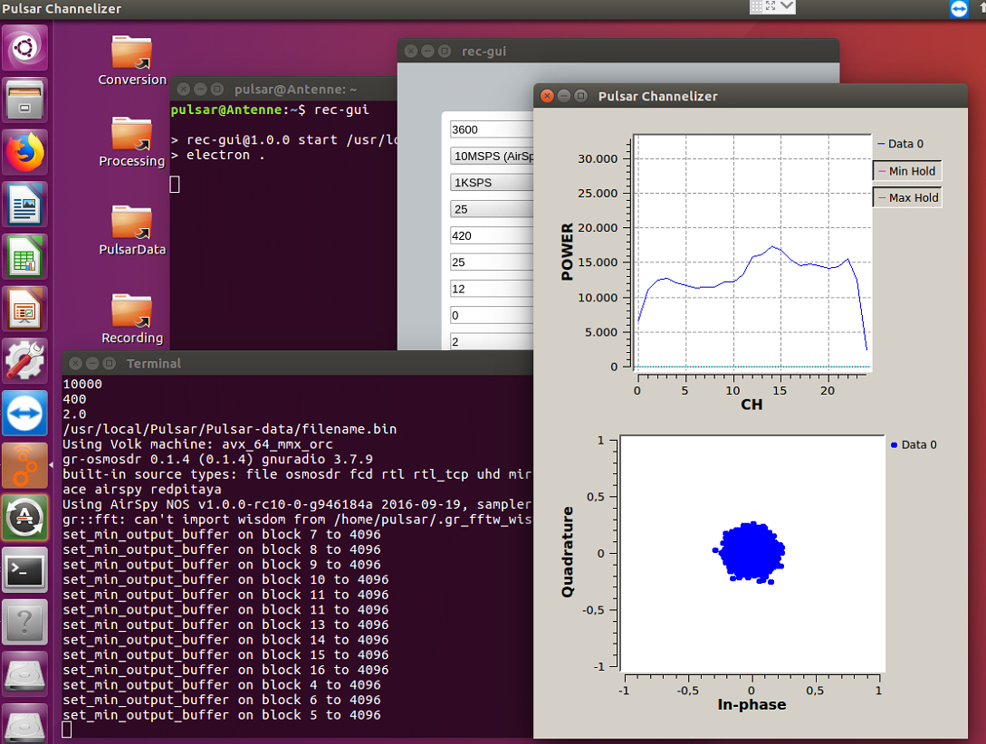
Once the recording is started you should see the I/Q cloud and the power per channel graphs.

Make sure that the I/Q cloud is neither too small or saturated (it should be approximately like in the picture above). If it's not, tweack the RF/IF/BB gains until you reach a good I/Q amplitude (see above).

Conversion

When the recording is complete you have to convert the .bin file to a .fil file (format that is used by professional pulsar analysis softwares like presto or sigproc).
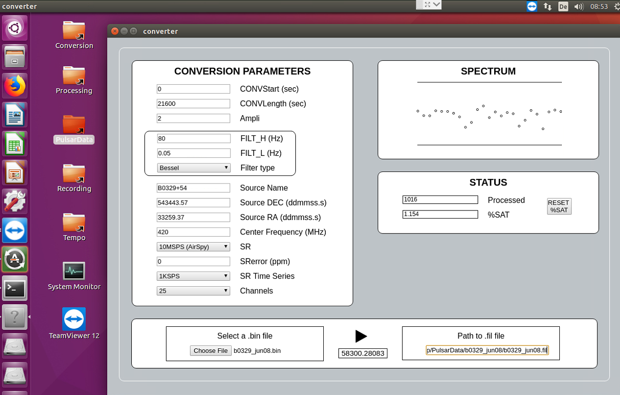
In order to do that just type in the terminal

bin2fil

and again set the values of the conversion so that they're coherent with the value of the recording.

CONVStart / CONVLength - the tool will convert from CONVStart CONVLength seconds
Ampli - scale factor (tweack until you get few % of saturation)
FILT_H / FILT_L - The filters value are calculated approximately by the formulas

FILT_H ~ 600/(pulse width of pulsar) (ms)
FILT_L ~ (pulsar frequency)/20 up to (pulsar frequency)/10

Source Name - name of the pulsar (written in .fil header)
Source DEC - declination of the pulsar (written in .fil header)
Source RA - right ascension of the pulsar (written in .fil header)
Center Frequency - center frequency on the acquisition (written in .fil header)
SR - sample rate of the acquisition (written in .fil header)
SRerror - frequency error in ppm of the dongle
SR Time Series - sample rate of the time series (written in .fil header)
Channels - number of channels (written in .fil header)

All the values that are written in the .fil header must be consistent with the recording values.

To change default values for the input fields edit default.conf.xml in the Conversion folder

Setting up Tempo

Tempo is a program for the analysis of pulsar timing data. Pulsar rotation, astrometric, and binary parameters are deduced by fitting models to pulse times of arrival measured at one or more terrestrial observatories. (more info)

To set up Tempo for your radiotelescope open the Tempo folder o Desktop and open obsys.dat; here you can find informations about the radiotelescopes that are availables and you can add a line containing data from your location. Here's a printout of the last lines of obsys.dat in the distribution:

(LATITUDE)    (LONGITUDE)     (ALTITUDE)        (NAME)            (ID)  (INITIALS)
(ddmmss.ss)   (ddmmss.ss)     (m)

355615.0      1060230.0       200.              K5SO              j     SO
440515.0      -102750.0       300               IW5BHY            k     BY
481607.0      -130235.0       300               OE5JFL            l     JF

Once you have done that you have to open the tz.in file and modify the following values:

l 6 480 5 422
  Name     Nspan Ncoeffs (1st line: defaults for nsite,maxha,nspan,ncoeff,freq)
------------------------
0329+54

the first character that is the telescope id defined in obsys.dat
the frequency (in the example is 422 MHz)
the name of the pulsar you want to calculate for (in the example 0329+54)

Analysis

First of all go to the folder containing the .fil file (b0329_test.bin) and open a terminal. Before the folding you should look for RFI in the recording. In order to do that you can run the following command

rfifind -o mask -time 1 -timesig 4 -freqsig 15 -chanfrac 1 -intfrac 1 b0329_jun08.fil

you can get information about these parameters with rfifind. During this process will be created some 'mask' files that indicates if and where are RFIs.

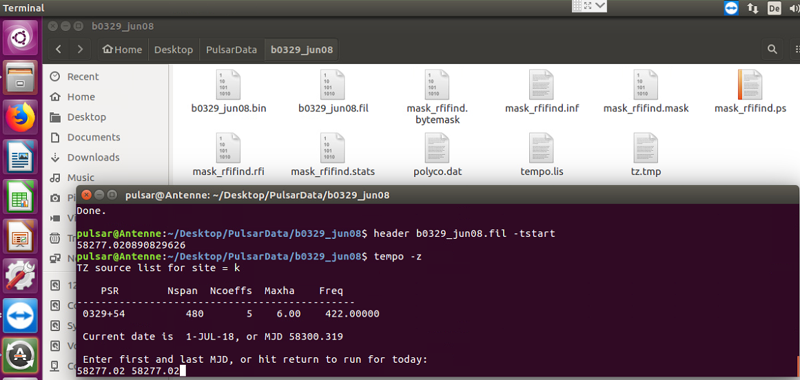
For calculating the pulsar period we need MJD time for the recording. We get this parameter by typing

header b0329_jun08.bin –tstart

In our case the result is 58227.02. By the way the header command is a very useful tool to display information contained in te header of the .fil file; the syntax is header filename.fil.

Now you need to calculate the polynomial curve that represent the change in time of the frequency. To do that type

tempo -z

and you will be asked for the first and last value of MJD; insert the value calculated previously.

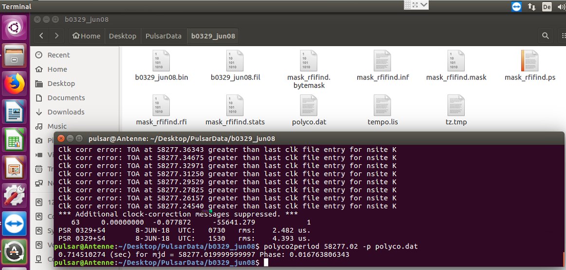
This will create some files, like ployco.dat or tempo.lis

To calculate the period of the pulsar you can use

polyco2period 58277.02 -p polyco.dat

this will output the period that you have to copy somewhere for further elaborations.

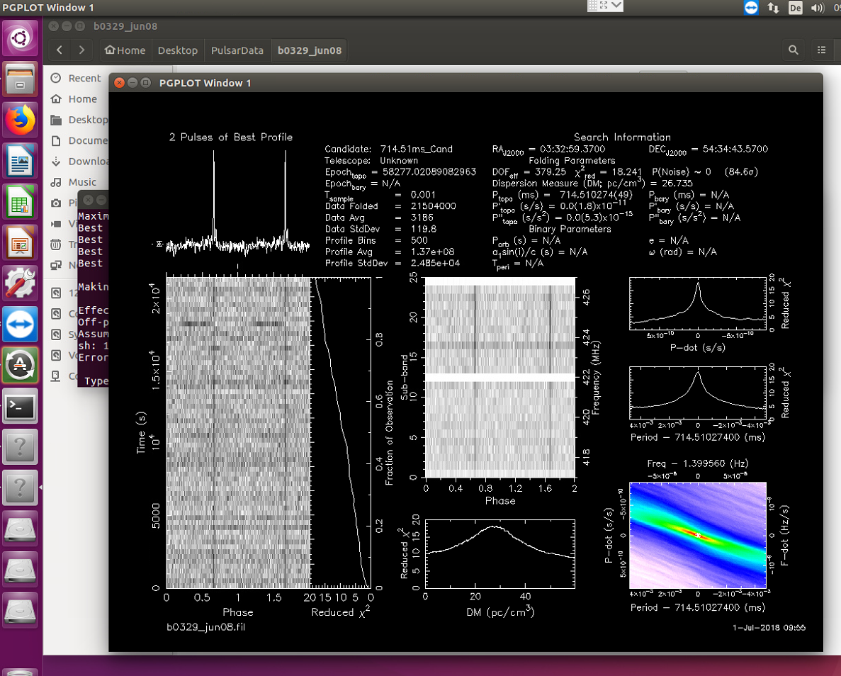
To fold the data use the command

prepfold -nsub 25 -n 500 -topo -dm 26.75 -nosearch -mask mask_rfifind.mask –p 0.714510274  -fine b0329_jun08.fil

again you can get information about these parameters with prepfold.

If all went good you should finally see the result!

You can now convert the .ps file into an image by opening it in GIMP, import with resolution 300 and export it as a png (or whatever image format you want) file.

For testing we can provide sample .bin files and/or .fil files.

Good luck!

gio54321/pulsar-distro-guide