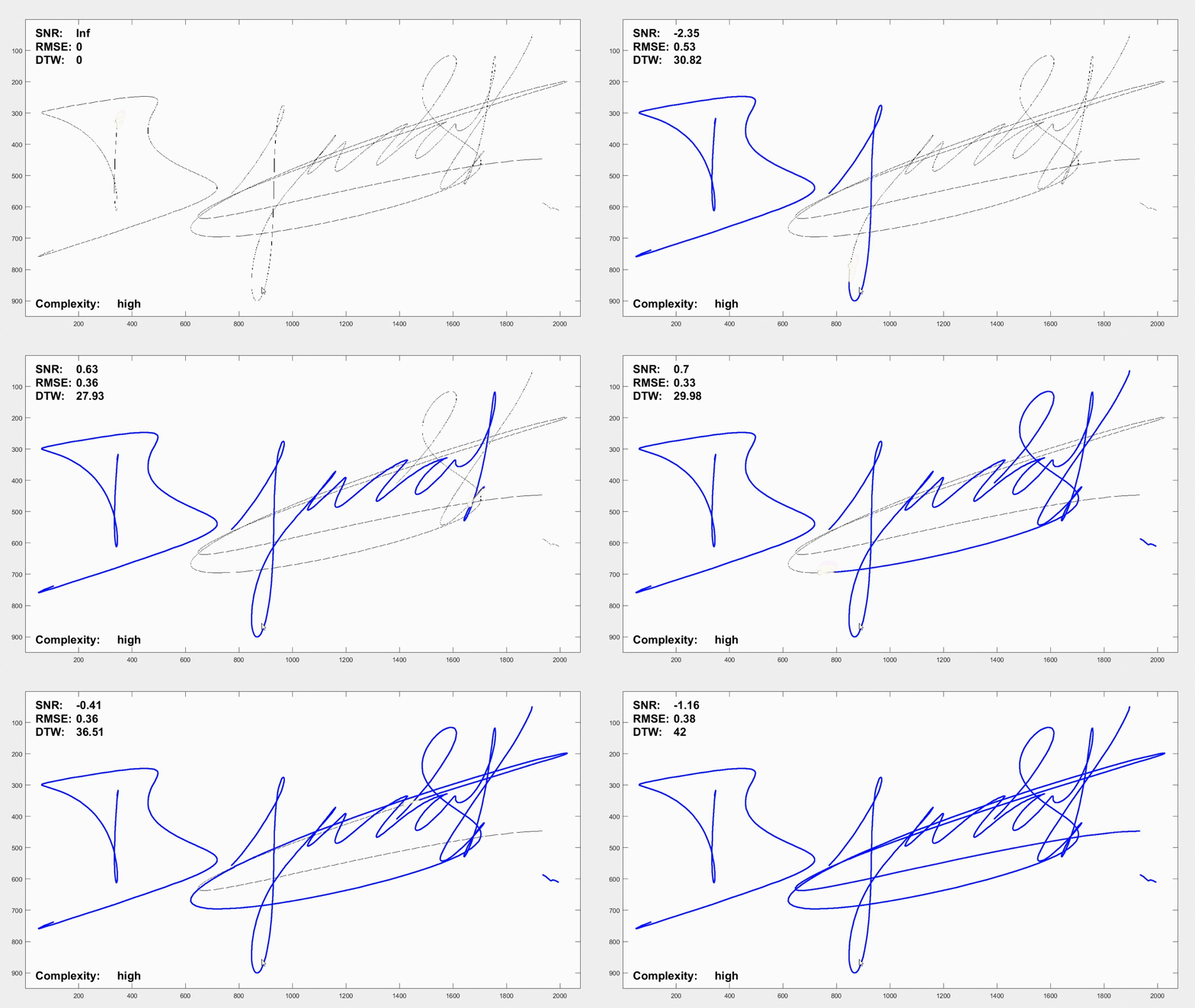
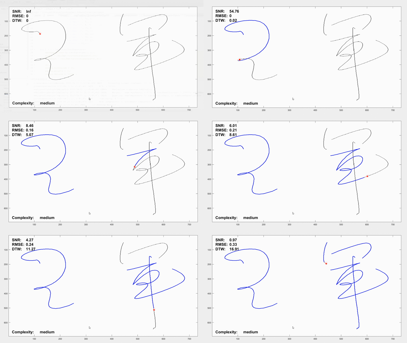
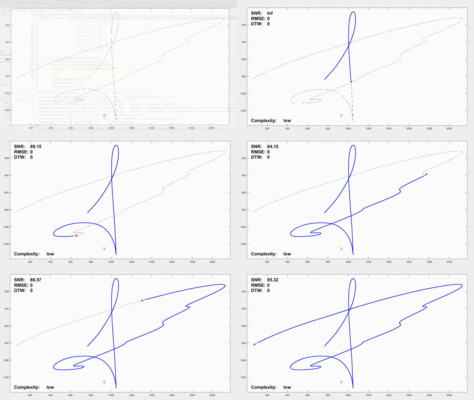
Writing Order Recovery in Complex and Long Static Handwriting

This repository contains a MATLAB implementation for our paper.
If you find this code useful in your research, please consider citing:

    @article{diaz2021wor,
      title={Writing Order Recovery in Complex and Long Static Handwriting},
      author={Diaz, Moises and Crispo, Gioele and Parziale, Antonio and Marcelli, Angelo and Ferrer, Miguel A.},  
      journal={International Journal of Interactive Multimedia and Artificial Intelligence},
      volume={X},
      number={X},
      pages={1--14},
      year={2021},
      publisher={UNIR},
      doi = {To appear}
    }

Here are examples on how our system recover trajectories of some samples. See the full video here.

High complexity

More examples

Medium complexity

Low complexity

Installation
Run the code
- Run the wor code
- Run the full code
Algorithm Threshold and options configuration

Installation

Clone the code on you local machine and run src/main.m or the src/main_full.m script. Please note that the working directory has to be src (not the root folder).

Requirements

You must have Matlab version 2016.a or major to run this code.

Run the code

The code is structured this way:

src/main.m contains the code for recovering the writing order starting from an image. It is aimed at those who want to just use the code to perform the writing order recovery on an image. See this section.
src/main_full.m contains the code for recovering the writing order of an image with the comparison with the online version to research purposes. It allows replicating our previous experiments and it is aimed at those who want to explore our work and change some parameters or just do research starting from this code. See this section.

Remember anyway you have to run the following code first:

clearvars -except thresholds weights
restoredefaultpath
addpath(genpath('./'))

It is needed to make Matlab aware of all the functions in the folder. You need to run it in src, as usual.

Run the wor code

The code below, in the main.m file, allows you to run the writing order recovery on an image.

imagepath = '../databases/examples/high/c-092-02__thin.png';
% doplot => [OPTIONAL] 0 if you don't want plot / 1 otherwise;
% config => [OPTIONAL] for config see below
[x, y, wor_result] = wor(imagepath, doplot, config)

wor is a function that accepts three inputs:

the image path;
an optional flag for showing the dynamic plotting of the trajectory on the image, as shown in the demo;
an optional additional configuration, if you want to change it. For the additional configuration take a look of the src/Execution/Options/configuration.m file.

wor function is composed of these step:

function [x, y, wor_result] = wor(imagepath, doplot)
%% CONFIGURATION AND IMAGE LOADING
options = configuration();
data = loadData(options, imagepath);
%% POINT CLASSIFICATION
% - Image analysis, point classification and cluster detection
[image, clusters] = pointClassification(data, options);
%% LOCAL EXAMINATION
% - Skeleton correction and cluster processing
[image, clusters] = localExamination(image, clusters, options);
%% GLOBAL RECONSTRUCTION
% - Initial point detection and trace following
[x, y, wor_result] = globalReconstruction(image, clusters, data, options);

if doplot == 1
   drawTrajectory_dynamic(image.bw, x, y)
end

end

Here, the default options are used. These are the parameters that, according to us, best guarantee the recovery of a handwritten sample. You may only specify if you want to plot the recovered trajectory or not.

Run the full code

% OPTIONS - Required. See the "Algorithm thresholds and option Configuration" section below for more details.
[image, clusters, unfolder, data, results] = wor_results(options);

that takes as input where wor_results is defined as follows:

function [image, clusters, unfolder, data, results] = wor_results(options)

%% OPTIONS INITIALIZATION
% - Algorithm thresholds and weights initialization
options = configuration(options);

%% DATA LOADING AND INITIALIZATION 
% - Image reading and data loading
[data, options] = loadData(options);

%% POINT CLASSIFICATION
% - Image analysis, point classification and cluster detection
[image, clusters] = pointClassification(data, options);

%% LOCAL EXAMINATION
% - Skeleton correction and cluster processing
[image, clusters] = localExamination(image, clusters, options);

%% GLOBAL RECONSTRUCTION
% - Initial point detection and trace following
[x, y, wor_results] = globalReconstruction(image, clusters, data, options);

%% COMPUTING RESULTS
% - Process evaluation and drawing unfolded trace
results = worEvaluation(image, clusters, wor_results, data, options);

%% DRAWING RESULTS
% - Drawing unfolded trace, components
drawSignatureResults(image, clusters, unfolder, data, options, results);

%% CLEARING ENVIRONMENT
% - Clearing data, options, unfolder and so on
cleanEnvironment(image, data, clusters, unfolder, options);

end

Algorithm Threshold and options configuration

In this section, the threshold and the weights used in the algorithm decisional part are defined. For more information see the paper attached. Also, the code options for logging, debug and execution are defined.

% Thresholds and weight for algorithm
options.thresholds = [];     % set default. see Execution/Options/Thresholds.m for other details.
options.weights = [];        % set default. see Execution/Options/WeightedVote.m for other details.
    
% Signature - Overwrite these values if you want to use the wor_results function
options.imagebasepath = '../databases';  % database base path 
options.databaseName = '';    % database name that has to be in the databases folder
options.writer = NaN;         % writer number that has to be in the database name folder
options.signature = NaN;      % signature number that has to be in the writer folder


% Additional options
options.plot = true;               % if true, it enables all plots
options.real = false;              % if true, it elaborate also the skeleton. The 'skeletonized' version is needed 
options.computeResults = false;    % if true, it compute result with online. Note that the 'online' version is needed
options.saveResults = false;       % if you want to save the results
options.saveDrawings = false;      % if you want to save also the drawings
options.loglevel = 'OFF';    % As LogLevel, you can choose: ALL; TRACE; DEBUG; INFO; WARNING; ERROR; CRITICAL; OFF
options.debug = false;       % if true, it executes also the debug code
options.cleanAfterExecution = false;   % if true, it cleans environment. Needed for experiments (successive executions in a loop)

For the execution, we could choose for different strategies:

ESTNC: Estimed Starting Points Nearest Criteria -> we estimate the components starting points and we choose the next through the Nearest Criteria (by taking the end point with the minimum distance).
RSENC: Real Starting/Ending Point Nearest Criteria -> we take the starting/ending points location from the real reference (the 8connected version) and we choose the next through the Nearest Criteria (by taking the end point with the minimum distance). You need the online version of the specimen.
RSEOC: Real Starting Point Ordered Criteria -> we take the starting/ending points location from the real reference(the 8connected version) and we choose the next by looking at the reference (we have an ordered set of starting points). You need the online version of the specimen.
ALL: all the previous strategies, together. You need the online version of the specimen. If you don't know or do not have the onli version, keep 'ESTNC', or use the wor function instead.

options.version = 'ESTNC' % [RSENC, RSEOC, ALL]

gioelecrispo/wor