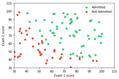
Predict chance of getting admission into University

Problem statement

Determine each applicant's chance of admission based on their results on two exams. You have historical data from previous applicants that you can use as a training set for logistic regression. For each training example, you have the applicant's scores on two exams and the admissions decision.

Dataset

Exam 1 Score	Exam 2 Score	Admission
34.62365962451697	78.0246928153624	0
30.28671076822607	43.89499752400101	0
60.18259938620976	86.30855209546826	1

Now we have to predict chance of getting admission into university (including which is not mention in our example dataset).

Note:This problem statement and dataset is from coursera Andrew ng machine learning Coursework

Dependencies

jupyter
scipy
numpy
matplotlib

Install dependencies using pip

import numpy as np
import matplotlib.pyplot as plt
# supress scientific value
np.set_printoptions(suppress=True)

data = np.loadtxt("ex2data1.txt",dtype=np.float64,delimiter=",")
data[0:5,::]

array([[ 34.62365962,  78.02469282,   0.        ],
       [ 30.28671077,  43.89499752,   0.        ],
       [ 35.84740877,  72.90219803,   0.        ],
       [ 60.18259939,  86.3085521 ,   1.        ],
       [ 79.03273605,  75.34437644,   1.        ]])

# split data into features and outputs
X = data[::,0:2]
Y = data[::,-1:]

# Visualising the Dataset
X_get_admit = np.select([Y==1],[X])
X_not_admit = np.select([Y==0],[X])
plt.xlabel("Exam 1 score")
plt.ylabel("Exam 2 score")
plt.xlim(30,110)
plt.ylim(30,110)
plt.scatter(X_get_admit[::,0:1],X_get_admit[::,-1:],label="Admitted",color="#2ecc71" )
plt.scatter(X_not_admit[::,0:1],X_not_admit[::,-1:],label="Not Admitted",color="#e74c3c")
plt.legend(loc = "upper right",frameon=True)
plt.show()

# sigmoid function
def sigmoid(Z):
    return (1/(1+np.exp(-Z)))

# hypothesis with sigmoid
def hypothesis(X_bias,Theta):
    #here Theta is 1d convert it into 2d
    hx = X_bias.dot((Theta.reshape((1,3))).transpose())
    return sigmoid(hx)

# cost function
def cost(Theta,X_bias,Y):
    m,n = X_bias.shape
    hx = (hypothesis(X_bias,Theta))
    first = np.multiply(-Y,np.log(hx))
    second = np.multiply((1-Y),np.log(1-hx))
    return (1.0/m)*np.sum(first - second)

m,n = X.shape
Theta = np.zeros(n+1)
X_bias = np.ones((m,n+1))
X_bias[::,1:] = X
cost(Theta,X_bias,Y)

0.69314718055994529

# gradient finding method used for advance optimization algorithm
def gradient(Theta,X_bias,Y):
    m,n = X_bias.shape
    grad = np.zeros(n) 
    hx = hypothesis(X_bias,Theta)
    error = hx -Y
    for i in xrange(n):
        element = np.multiply(error,X_bias[:,i].reshape((100,1)))
        grad[i] = np.sum(element)/len(X_bias)
    return grad    
gradient(Theta, X_bias, Y)

array([ -0.1       , -12.00921659, -11.26284221])

import scipy.optimize as opt
result = opt.fmin_tnc(func=cost, x0=Theta, fprime=gradient, args=(X_bias,Y))
print result

(array([-25.16131862,   0.20623159,   0.20147149]), 36, 0)

Theta = result[0]
print Theta # result is 1d array convert it to 2d array for bug free calculation
print Theta.shape

[-25.16131862   0.20623159   0.20147149]
(3,)

cost(Theta, X_bias, Y)

0.20349770158947456

hx = hypothesis(X_bias,Theta)
# assume 1 if hx >= 0.5 and assume 0 if hx < 0.5
threshold = 0.5
prediction = np.select([hx >= threshold, hx < threshold],[1,0])
final_error =  (np.sum(np.absolute(Y-prediction))/len(X))*100
print 'accuracy', (100-final_error),'% with threshold ',threshold

accuracy 89.0 % with threshold  0.5

# lets try with different threshold
threshold = 0.3
prediction = np.select([hx >= threshold, hx < threshold],[1,0])
final_error =  (np.sum(np.absolute(Y-prediction))/len(X))*100
print 'accuracy', (100-final_error),'% with threshold ',threshold

accuracy 92.0 % with threshold  0.3

girishkuniyal/Predict-chance-of-getting-admission

Predict chance of getting admission into University

Problem statement

Dataset

Dependencies