
Analytical model for analyzing the mechanical properties of tubular braided composites
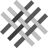
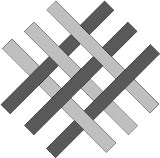
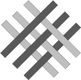
Braided Composites can be manufactured in several different braiding patterns: Diamond (1/1), Regular (2/2) and Hercules (3/3). Examples of the different patterns are shown below
Current work on braided composites typically focuses on one specific pattern. The goal of this model is to be able to predict the mechanical properties of all the available braiding patterns. Another limitation of current studies that examine braided composites is that most researchers do not take into consideration the geometry and the physical process of manufacturing composite braids. Both braid geometry and the manufacturing process has an effect on the mechanical properties of tubular braided composites. No software tools are currently freely available for predicting the mechanical properites of braided composites.
The user interface for the Braided Composite Analytical Model is show below
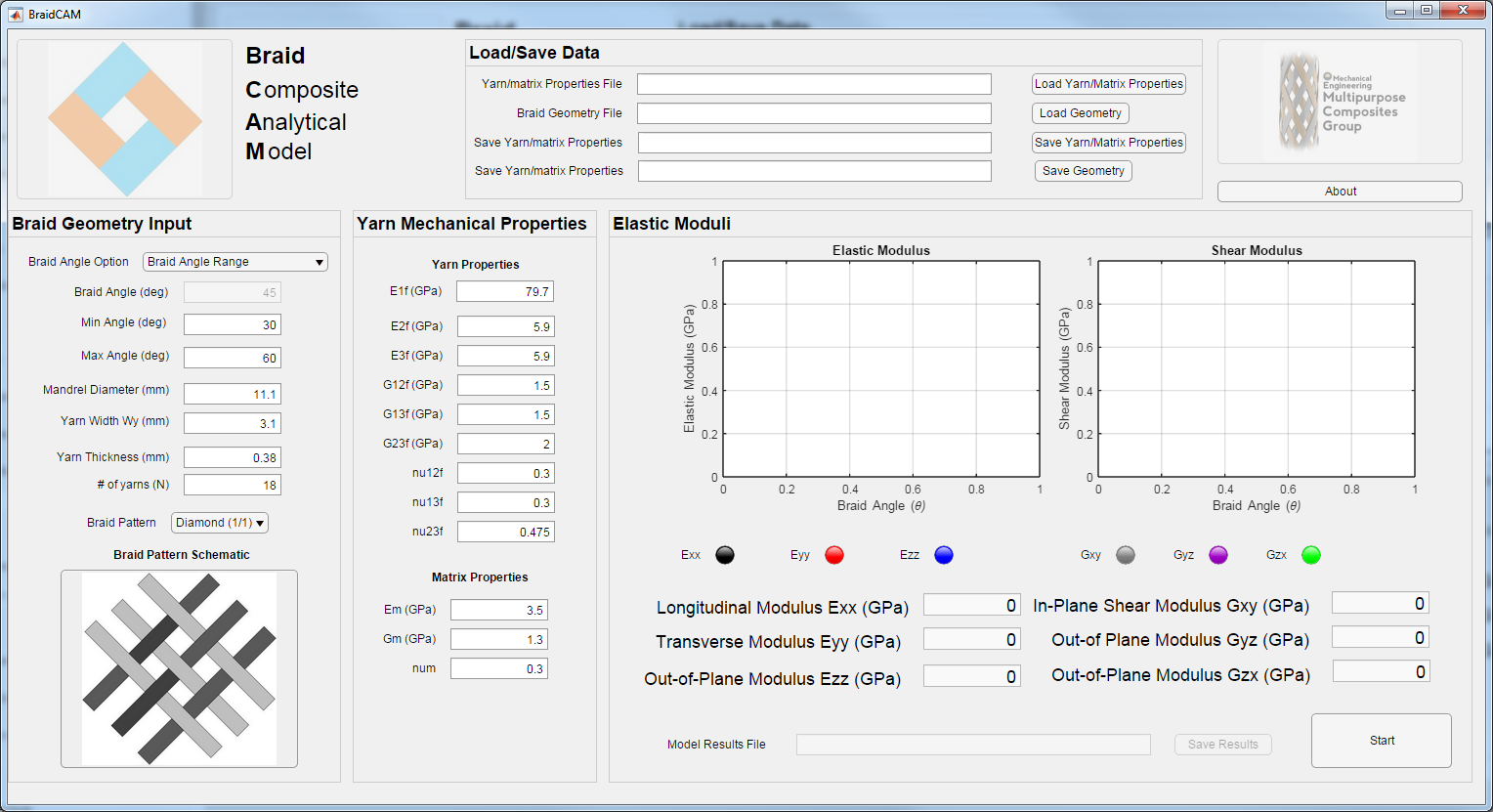
The user interface allows for the geometric properties as well as mechanical properties of yarns and matrix used to create composite braided to be easily adjusted.
The user can load and save braid geometries and yarn/matrix mechanical properites using the Load/Save Data panel.
Once the desired geometry and mechanical properties have been entered the 'Start' button is selected to display the resulting mechanical properties.
There are two options for displaying the mechanical properties of braided composites: Braid Angle Range and Single Braid Angle
The option "Braid Angle Range" will create two plots which show the effect of braid angle on elastic and shear moduli
The option "Single Angle" will display the mechanical properites for a specific braid angle.
Braid model settings can be saved using the 'Save Results' button.
The save results button will save the entered braid geometry, yarn/matrix mechanical properties and will save the braid model results to a single CSV file.
The program can be installed using several approaches
The Braided Composite Analytical Model (BraidCAM) has been developed using the Matlab App Developer program which is available in Matlab 2016a The Braided Composite Analytical Model can be installed by selecting the file Braid CAM.mlappinstall This will add the Braided Composite Analytical Model to the Apps ribbon bar in Matlab
The Briad CAM can be run as an executable file. Select the file BraidCAM.exe to install the program. A MATLAB runtime engine will be required to run this file. The runtime engine will automatically download the first timee the executable is run. Once the runtime engine has been isntalled the file BraidCAM.exe can be used. Once installed, this option will not require MATLAB.
The main braid model has been written as matlab m-file functions. The m-file functions can be used within the MATLAB environment without the need of a graphical user interface. In order to run the braid model the function braidModel.m will be used. The input and output of the braidModel function is shown below. The function will return the mechanical properties of a composite braid.
[Ex, Ey, Ez, GxyCombined, GyzCombined, GzxCombined] = braidModel(S, Sm, angle, n, r0, a, b, beta, braidType)
Example inputs for the briadModel function are shown below
%The following braid patterns can be analyzed using this method: %1) diamond braid pattern (1/1) %2) regular braid pattern (2/2) %3) Hercules braid pattern (3/3) %**************************************************************************
%Initial parameters for braid geometry % a = 0.38; %yarn thickness % b = 3.1; %yarn width % D = 11.1; %mandrel diameter % t = 2*a; % braidType = 3; %type of braid see above
% R = D/2; % mandrel size mm % r0 = R+a; % nomial braid radius mm
% Define the braid angle between 30 and 60 degrees
% angle = linspace(30,60,100); % %Define braiding machine parameters % n = 18; %number of carriers % Nc = 2n; % total number of carriers % beta = 2pi / n; % braid shift angle (rad) % % Material Properties % Matrix material properties % Em = 3.5; % Gm = 1.3; % num = 0.3;
% Vf = 0.6; % Vv = 4.35 / 100; % %Vv = 0; % Vm = 1 - Vf - Vv % ************************************************************************* % %Fiber, Matrix and Fiber+Matrix Material Properties % *************************************************************************
% Ef1 = 130; % Ef2 = 7.3; % Ef3 = Ef2; % Gf12 = 2.86; % Gf13 = Gf12; % nuf12 = 0.35; % nuf13 = nuf12; % nuf21 = nuf12*(Ef2/Ef1); % nuf31 = nuf12*(Ef3/Ef1); % nuf23 = 0.1; % nuf32 = nuf23*(Ef3/Ef2); % ************************************************************************** % %Source: Kevlar/epoxy %***************************************************************************
% E1 = 79.7; % E2 = 5.9; % E3 = E2; % G12 = 1.5; % G13 = G12; % eta23 = (3 - 4num + (Gm / Gf12)) / (4(1-num)); % G23 = (Gm*(Vf + eta23*(1-Vf))) / (eta23*(1-Vf) + Vf*(Gm/Gf12)); % nu12 = 0.3; % nu13 = nu12; % nu23 = (E2/(2G23)) - 1; % nu21 = nu12(E2/E1); % nu31 = nu13*(E3/E1); % nu32 = nu23*(E3/E2);
% initial transversely isotropic compliance matrix for yarns+epoxy % S = [1/E1 -nu21/E2 -nu31/E3 0 0 0;... % -nu12/E1 1/E2 -nu32/E3 0 0 0;... % -nu13/E1 -nu23/E2 1/E3 0 0 0;... % 0 0 0 1/G23 0 0;... % 0 0 0 0 1/G13 0;... % 0 0 0 0 0 1/G12];
% initial compliance matrix for epoxy % Sm = [1/Em -num/Em -num/Em 0 0 0;... % -num/Em 1/Em -num/Em 0 0 0;... % -num/Em -num/Em 1/Em 0 0 0;... % 0 0 0 1/Gm 0 0;... % 0 0 0 0 1/Gm 0;... % 0 0 0 0 0 1/Gm];