Introduction

Ecosystems are inherently dynamic---the abundance and composition of different species at different places are constantly changing over time. Understanding how assemblages of species interact, change, and persist over time is one of the foundational goals of ecology as a science. At the same time, humans are radically impacting ecosystem dynamics through land-use and climate change, and adapting to and mitigating this change is essential to maintain the ecosystem services humanity relies upon [@Cardinale2012BioLos]. Being able to detect changes in biodiversity, attribute them to human and natural drivers, and forecast their future dynamics is crucial to maintaining biodiversity and the services it provides to humans [@Gonzalez2023FraDet]. However, ecosystems are perhaps the prototypical example of a complex adaptive system [@Levin1998EcoBio], meaning their dynamics are the product of a vast number of interconnected processes, many of which are inherently latent. If that were not enough, sampling of ecosystem dynamics as it exists is inherently incomplete and sparse in both space and time [@Hughes2021SamBia]. These factors together make the inference and forecasting of ecosystem dynamics quite difficult, imposing intrinsic limitations on prediction [@Beckage2011LimPre; @Pennekamp2019IntPre; @Petchey2015EcoFor]. Still, reliable forecasts of biodiversity and ecosystem dynamics are essential to guide decisions dedicated to mitigating and adapting to this change [@Urban2016ImpFor].

This need has resulted in efforts to develop a Global Biodiversity Observation System (GBiOS; @Gonzalez2023GloBio), modeled off of the Global Climate Observation System (GCOS). Part of the success of GCOS can be ascribed to its widespread adoption of standards and unified methods for modeling. There have been similar proposals for a unified modeling platform for biodiversity [@Urban2022CodLif], though this is largely impeded by the culture of ad-hoc model development and poorly adopted standards for data formatting and availability [@Poisot2019EcoDat]. A further difficulty is that in ecology, we also have no universal governing equations of ecological dynamics. Though there is universality in the fundamental forces driving the abundance and distribution of species across space [@Vellend2010ConSyn], these forces can manifest themselves in different ways, e.g. different types of functional responses in consumer-resource systems [@Holling1966FunRes]. So although the processes are universal, the balance of each of these processes manifested in a particular natural system is always going to be latent and require inference from data. This raises many questions: if we collect a time-series of a consumer-resource system, how then do we decide which functional response is “best” to forecast these species into the future? How can we be sure our data is even sufficient to distinguish between different dynamic regimes in the first place? What is the forecasting horizon for different ecological and evolutionary processes? And how do we ensure we propagate the uncertainty in our data into our projections to best inform decision making? These questions become even more complex when we consider that all ecological processes take place across space, where dispersal and heterogeneity in environmental conditions further complicate how these dynamics unfold.

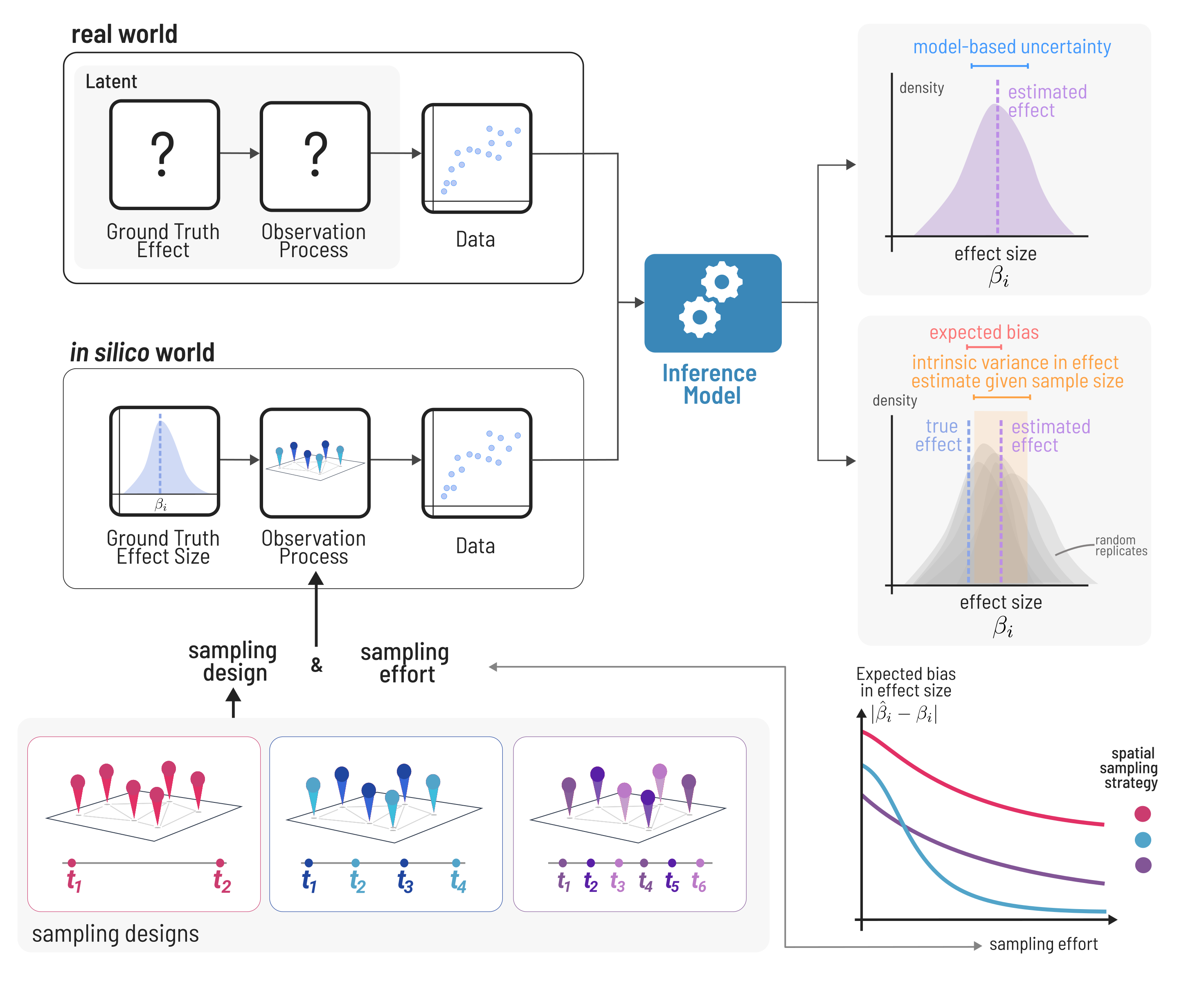
Biodiversity data is inherently sparse and biased [@Hughes2021SamBia], and this can lead to misleading or outright wrong conclusions due to underpowered statistical inference [@Leung2020CluCat]. In many scientific and engineering fields, it is standard practice to test any tools used for inference on simulated data before applying them to real data. This assures our inference is a robust reflection of the data and not providing erroneous results due to bugs in the inference code, or underpowered samples leading to either type-i or type-ii error. When using simulated data, we are sure of the “ground-truth” processes and known level of measurement error behind the data, so we can assess how well the given method is by comparing its inference to the known values (Figure @fig:inference). This is especially important for ecology, where our data is inherently sparse---Earth’s biosphere is very large and complex, there are millions of species undergoing dynamics in space and time, and we can only sample tiny snippets in time. The extent to which monitoring programs can cover all of this is limited practically by funding and human resources and time. The data we can collect is further biased by the spatial locations it was collected and unavoidably contains measurement error. We can never be certain of the “ground truth” driving community dynamics in nature. So, after collecting a dataset, we can never know if our statistical analyses we employ would be capable of capturing an effect if it was real. Typically power-analyses used to address this problem (e.g. @Green2016SimPac) relate sample size to properties of the statistical model itself (i.e. the probability of capturing a ‘significant’ effect in a linear model), rather than being based on the underlying mechanisms that generate the data (although see @Tucker2021EffSam as an example).

$Conceptual figure outlining the benefits provided from in silico power analyses on mechanistic models. In the top left, we see the pipeline from which known “ground truth” statistical effect $\beta_i$ becomes data in both the real world and in a simulated context. On the top right, we see the resulting information when data is obtained from the real world as opposed to repeated in silico simulations. In the case of in silico simulation, we have full information about the generating process, the sampling process (note the 3 sampling designs (bottom) involve the same number of total sampling events), and the amount of observational bias (in terms of both measurement error and temporal sparsity).$

Ecological processes are influenced by structured and random variation in the environmental conditions across space and time. The metacommunity framework [@Leibold2004MetCon] enables us to simultaneously consider the effects of the local environment, competition within populations, interactions between species, and dispersal of different species across space. The balance of the fundamental processes of demographic selection, drift, dispersal, and speciation [@Vellend2010ConSyn] leads to qualitatively distinct metacommunity paradigms [@Thompson2020ProMet]. Central to metacommunity theory is the abstraction that a landscape can be modeled as a set of discrete habitat patches connected via dispersal. The spatial graph framework allows us to apply tools from graph theory to understand landscape connectivity [@Dale2010GraSpa] and to model the heterogeneity in dispersal among species [@Albert2017AppNet; @Savary2023HetDis]. More generally, this enables us to represent metacommunity dynamics as dynamics on a network of networks, where within each spatial node there is a network of species, and the edges of the spatial graph model dispersal for each species [@Hutchinson2019SeeFor; @Pilosof2017MulNat].

Here, we present EcoDynamics.jl, a software toolkit for simulating a wide variety of models of population and community dynamics, both in isolation and as reaction-diffusion dynamics on spatial-graphs. EcoDynamics.jl enables both deterministic and stochastic dynamics, and has the potential for environmental covariates associated with nodes in the spatial graph to affect demographic parameters, enabling virtual experiments about the effects of spatial environmental variation on population and community processes. EcoDynamics.jl includes a rich library of models of population and community dynamics from the literature, and enables easy addition of customized models. This toolkit is built upon DifferentialEquations.jl [@Rackauckas2017DifJl], a high-performance library for ordinary and stochastic differential and difference equations---this integration enables differential equation solvers orders of magnitude faster than e.g. deSolver in R [@Rackauckas2017DifJl; @Rackauckas2019ConMod]. This also enables integration with other parts of the Julia ecosystem: Turing.jl [@Ge2018TurLan] or STAN.jl for Bayesian inference of differential equation parameters, and integrations with the rapidly burgeoning Scientific Machine-Learning (SciML) ecosystem [@Rackauckas2021UniDif], which enables inference by combining mechanistic, domain specific models (in the form of differential/difference equations) with data-driven models (neural networks) to account for and discover missing dynamics in complex systems [@Chen2019RevCom; @Cranmer2020DisSym; @Martin2018RevEco].

Aside from the sheer technical merits and advantages, EcoDynamics.jl also aims to serve as a platform that changes how we think about inference from data in ecology. When doing power analyses independent from the underlying mechanistic process, we lose important details about the underlying process generating the data, which is particularly relevant in planning the spatial and temporal aspects of sampling design. EcoDynamics.jl provides a “virtual laboratory” [@Grimm2013IndMod] for generating synthetic data under known conditions to aid in the planning and design of monitoring programs and the testing of scientific software for inference. We first provide an overview of the design of EcoDynamics.jl, and then explore a glimpse of the potential uses of the software using case-studies.

Software overview

Here we overview the design and common usage patterns in EcoDynamics.jl.

Why Julia?

Why write this library in Julia? It is true that Julia is not the most-adopted language among ecologists, although it offers several advantages for building a package with the design goals of EcoDynamics.jl. Julia is designed for scientific computing, and offers the syntax of a high-level language with the performance of a low-level, compiled language [@Bezanson2012JulFas]. A common pattern in developing software for scientific purposes is to first develop a prototype of the software in a high-level interpreted language (e.g. Python, R), and then to develop a second version for use at scale in a statically typed, compiled language (like C++ or FORTRAN).

These latter languages tend to have much higher performance and therefore for the many computationally intensive methods used in scientific computing, it is worth making the effort to port software into these more complicated languages. However, there is also a large downside here: languages like C++ are far less known among scientists (and particularly ecologists), and as more of the codebase used by scientists are written in lower-level languages, they can easily customize software for distinct purposes. The decreased extensibility of software tools caused by this two-language problem leads to bad outcomes: duplication of code and therefore effort, and furthers the proliferation of tools that use slightly different methodologies and standards to accomplish the same goal. Julia aims to solve the two-language problem by providing a language that is written like a high-level language, but uses a technique called just-in-time (JIT) compilation to compile Julia syntax into machine code that executes just as quickly as compiled C++.

The second reason is Julia’s state-of-the-art ecosystem for differential equations. Over the previous several decades of research in numerical computing methods for differential equations, many advances have been made for improving the speed, stability, and accuracy of the numerical integration methods. DifferentialEquations.jl provides a large library to modern integration methods and automates selection of the appropriate method based on the model specification [@Rackauckas2019ConMod].

Design Principles

While EcoDynamics.jl enables simulation of dynamics in a single place (locally), its main goal is to enable reaction-diffusion models on spatial graphs. EcoDynamics.jl is perfectly adequate for simulating the dynamics of single-species systems, the core design goals are motivated by simulating communities on spatial graphs, where environmental variation across each patch/node can independently influence the dynamics of each species. The design was also based around a particular emphasis on studying regime shifts in the resulting composition of species across space at different levels of neutral, niche, and dispersal processes. Using spatial graphs enables environmental heterogeneity via arbitrary environmental predictors and covariates, and explicit interspecific variation in response to the environment via species-specific traits.

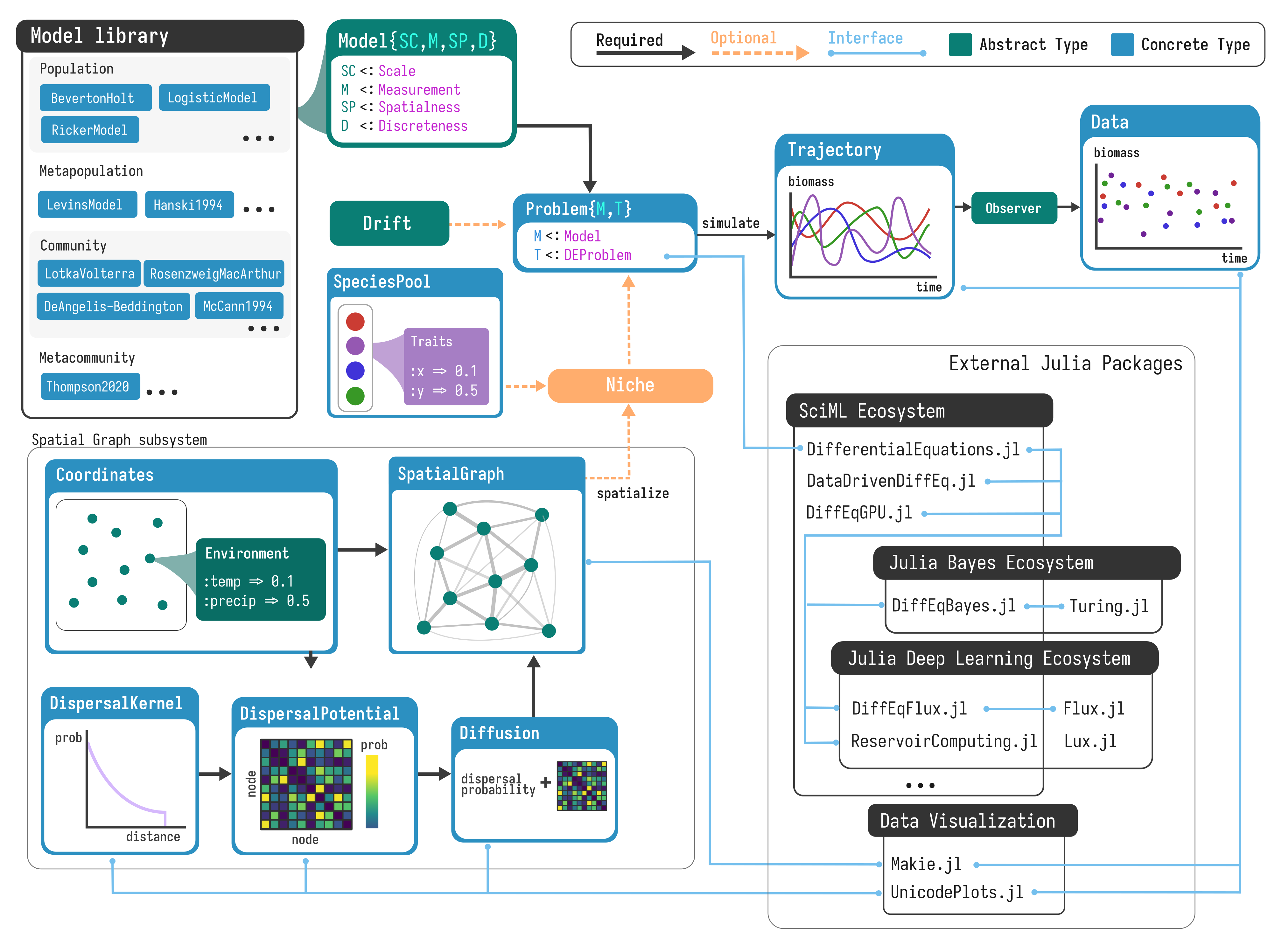
EcoDynamics.jl leverages Julia’s type system and multiple-dispatch system to use a common interface for constructing and running models. Models are built by calling them like a function, e.g. RosenzweigMacArthur(), Hanski1994(), etc., where parameters can be passed as named keyword arguments. Then, the pattern for constructing and running models follows the typical form (using Rosenzweig-MacArthur consumer-resource dynamics as an example):

rm = RosenzweigMacArthur()
prob = problem(rm)
trajectory = simulate(prob)

Multiple-dispatch is a feature of the Julia language that enables the same function name (e.g. problem or simulate above) to have different behavior based on the type of the inputs it is passed. This feature can be used in layers: for example, problem first dispatches (in the parlance of the Julia language) on the properties of models (described in the below section) which then pass specific objects and functions that enable the variety of models included in the library.

Why do we need a package for this purpose? This is the meta-question that underlies this manuscript. Why build a tool to do this---how much utility is gained by having a prewritten set of tools for reaction-diffusion dynamics on spatial graphs as opposed to an interested user implementing it from scratch? There is a fundamental point to be made about all (good) scientific software here: it should never be harder for a user, regardless of programming experience in a particular language or in general, to learn to use a package to do something than it would be to write code to do that something from scratch. If this is not the case, the package is either unnecessary, bad, or both. What, then, should a good package accomplish? (1) Minimum friction from going to nothing to a minimum working example. This is where first impressions are made, and first impressions count a lot in software. (2) Documentation matters a lot, but that isn’t something I can address in this paper outside of linking to it and saying “it has good documentation”. (3) Standardization of tools and methodology. If a particular abstraction for modeling a system is common enough, there is going to be a ton of wasted effort in the duplication of code for the same purpose, and it becomes more likely that some instances of this duplicated code will contain bugs. wIf many people are compelled to build the same thing independently, there is clearly some level of community demand for it. The point of open-source software is that the interface can be adapted to make the most sense to the most people. I think there is a sizable research community that wants to be able to run models like this without having to build the entire thing from scratch. There are arguably similar tools that exist, e.g. rangeshiftr, but these tools are limited in their extendability. One of the core design goals is extensibility first, and that should make this appealing to the general community of researchers interested in these types of models.

Finally, one of the core goals of EcoDynamics.jl is to be extendable---that is it will almost always be easier for a user to add a new model or additional feature than to rewriting a new set of tools to reaction-diffusion dynamics on spatial graphs with the desired model/feature. EcoDynamics.jl manages this by providing a uniform API for all models in the library, and extending a model is as straightforward as defining the model struct and implementing the ∂u method describing the rule to update from one timestep to the next. Extra methods for plotting and other utilities are optional, and are not required to get a model running from scratch.

Package Design

{#fig:design}

Models

Every model in EcoDynamics is associated with four properties that provide instructions to the package internals on how to simulate it. The first is the measurement, or the type of state space the model takes place in (biomass, abundance, and occupancy are what is currently supported). The second is the model's scale (population, community, metapopulation, or metacommunity)---note that this refers to the scale that a model was originally defined at, e.g. Lotka-Volterra is always a Community scale, regardless of whether it had been made spatial with spatialize. The third is the temporal domain, i.e. whether the model exists in discrete or continuous time. Finally, there is spatialness, which describes whether a model is associated with a spatial graph or is only at a single location.

Spatial Graphs and Reaction-Diffusion Models

Modeling patchy landscapes with spatial graphs has proven a useful abstract in ecology [@Dale2010GraSpa]. Although explicitly discretized Euclidean space has been used in ecological model (e.g. @Hastings1978GloSta), the complexity induced by this model of space, as well as the difficulty of adequate describing spatial heterogeneity in this framework, often makes the computational costs with this type of model not worth the benefit. In contrast, spatial graphs that explicitly represent heterogeneity in the environment and in dispersal have widespread utility in ecological modeling [@Hutchinson2019SeeFor; @Savary2023HetDis] and conservation [@Albert2017AppNet]. Spatial graphs can easily be adapted to simulate spatial ecological dynamics by adapting the reaction-diffusion framework [@Okubo1978DifEco], which is widespread for modeling processes with both spatial and local components across a wide-variety of domains, and which originated in its modern form for biology specifically (Turing’s model of morphogenesis; @Turing1952CheBas).

Reaction-diffusion dynamics follow the form

$$\frac{d\vec{N}}{dt} = g(f(\vec{N}))$$

where $\vec{N}$ is a vector where each element is a (not necessarily a scalar) measurement associated with each site, $f$ is a function that describes the local dynamics and applies that same transformation to each element of $\vec{N}$, and $g(\vec{N})$ is a function that describes diffusion across space.

More specifically, in spatially continuous models of ecological dynamics (e.g. @Hastings1978GloSta), where each spatial location has a two-dimensional coordinate $\vec{x} = (x_i, y_i)$ associated with it, $g(x)$ is the Laplacian operator

$$g(\vec{N}) = D_i \nabla^2 N_i = D_i \frac{\partial^2 N_i}{\partial^2\vec{x}}$$

where $D_i$ is a diffusion coefficient associated with each species.

Analogously, reaction-diffusion dynamics can be described for spatial graphs by utilizing the Laplacian as it is defined on graphs---the matrix $\mathbf{L} = \mathbf{K} - \mathbf{A}$, where $\mathbf{K}$ is a matrix with the degree of each node $k_i$ on its diagonal, and $\mathbf{A}$ is the adjacency matrix [@Gibert2019LapMat]. The topology of the spatial graph can reveal considerable information about how the dynamics will unfold across space---the eigenvalue spectrum of the Laplacian governs key properties of the realized spatial dynamics [@Gibert2019LapMat].

A common method to describe dispersal probability between patches/nodes is using a dispersal kernel---a function $k$ that maps a physical distance $d$ to a probability that an individual will successfully disperse that distance. We propose a modification to dispersal kernels that makes them more naturally suited to diffusion dynamics on a graph. For each node in the spatial graph $i$ at coordinate $x_i$, we first compute the dispersal kernel matrix for each pair of patches, $K_{ij}$ as

$$K_{ij} = \begin{cases} k(|x_i - x_j|) \quad\ &\text{if}\ |x_i - x_j| < \epsilon \\ 0 &\text{else} \end{cases} $$

where $\epsilon$ is the maximum dispersal distance of the organism, and then renormalize across each row (where $i$ is the source of dispersal) to produce the dispersal potential $\Phi_{ij}$ as

$$\Phi_{ij} = \begin{cases} \frac{K_{ij}}{\sum_k K_{ik}} \quad\ &\text{if}\ \sum_k K_{ik} > 0 \\ 0 &\text{else} \end{cases} $$

This forms a categorical distribution for each node/patch $i$ that describes where individuals successfully dispersing from that patch are going to end up. To turn this into a full-fledged reaction-diffusion model, we need one more step, which is the probability that any given individual disperses durings its lifetime, $m$. This final step allows us to construct the diffusion matrix $D$ as

$$D_{ij} = \begin{cases} m_i \Phi_{ij} &\text{if}\ i\neq j \\ 0 &\text{if}\ i =j \end{cases} $$

which is a stochastic matrix (for each source patch $i$, the values over all possible targets $j$ forms a distribution), ensuring conservation of mass in the system. From this we can construct our diffusion functio $g(x_i)$ for each species $i$ as

$$g(x_i) = D_{(i)}^T f(N_i)$$

where $f(N_i)$ describes local dynamics.

Environmental heterogeneity

EcoDynamics enables heterogeneity in the environment by enabling covariates of arbitrary type to be associated with each node. Covariates can be ascribed to each node by providing a raster in the same spatial coordinate system, drawing randomly from a known distribution, generated via NeutralLandscapes.jl, or assigned manually. These environmental covariates have the potential to affect ecological dynamics when paired with a user provided niche function, which maps environmental covariates to unique values of the parameters for the dynamics model in each node/patch.

Inter-specific variation

Another crucial component to many models of community dynamics is variation in traits among species, which can affect both their impact on other species and effect of environmental conditions on dynamics. To accommodate for these effects in EcoDynamics.jl, we use a data type called SpeciesPool to store these trait values. As an example, in @Yodzis1992BodSiz, variation in the body-size is a crucial parameter required by the model. For this and similar models, a SpeciesPool is required as given a default value, but can be passed as a custom input to the constructor. Species specific traits are also passed as arguments to the niche function if it is provided as an input. This enables interaction between species traits and environmental conditions, including the possibility of more complex models of dynamics that include interactions between traits and the environment.

Stochastic Dynamics

Ecological dynamics are inherently stochastic---there is randomness in the variation of abiotic environmental conditions over time at different scales and intrinsic variation in ecological processes [@Melbourne2008ExtRis]. EcoDynamics.jl enables arbitrarily complex models of stochasticity via the state-of-the-art integrators for stochastic differential equations (SDEs) included with DifferentialEquations.jl [@Rackauckas2020StaHig; @Rackauckas2017AdaMet]. Similarly, within DifferentialEquations.jl discrete-time models can be either deterministic or stochastic, without using different integration algorithms.

Observation Models

Crucial to one of the core design goals of EcoDynamics.jl --- providing “ground truth” dynamics to benchmark inference methods --- is the ability to simulate the process of observation and its associated error. The processes that contribute to observation error in nature are numerous: there is of course standard measurement error, where the observed value of a variable is some amount different from the true value. But there are also biases imposed on data based on where and when they are collected. This highlights the importance of including a model of the observation process when doing power analysis using mechanistic models.

Case Studies

Here we present two sets of case-studies that demonstrate a variety of functionality in EcoDynamics.jl. The first pair of case-studies focuses on the spatial modeling features of EcoDynamics.jl, and the second pair focuses on doing inference from data using interfaces to tools for both Bayesian inference and Scientific Machine-Learning (SciML).

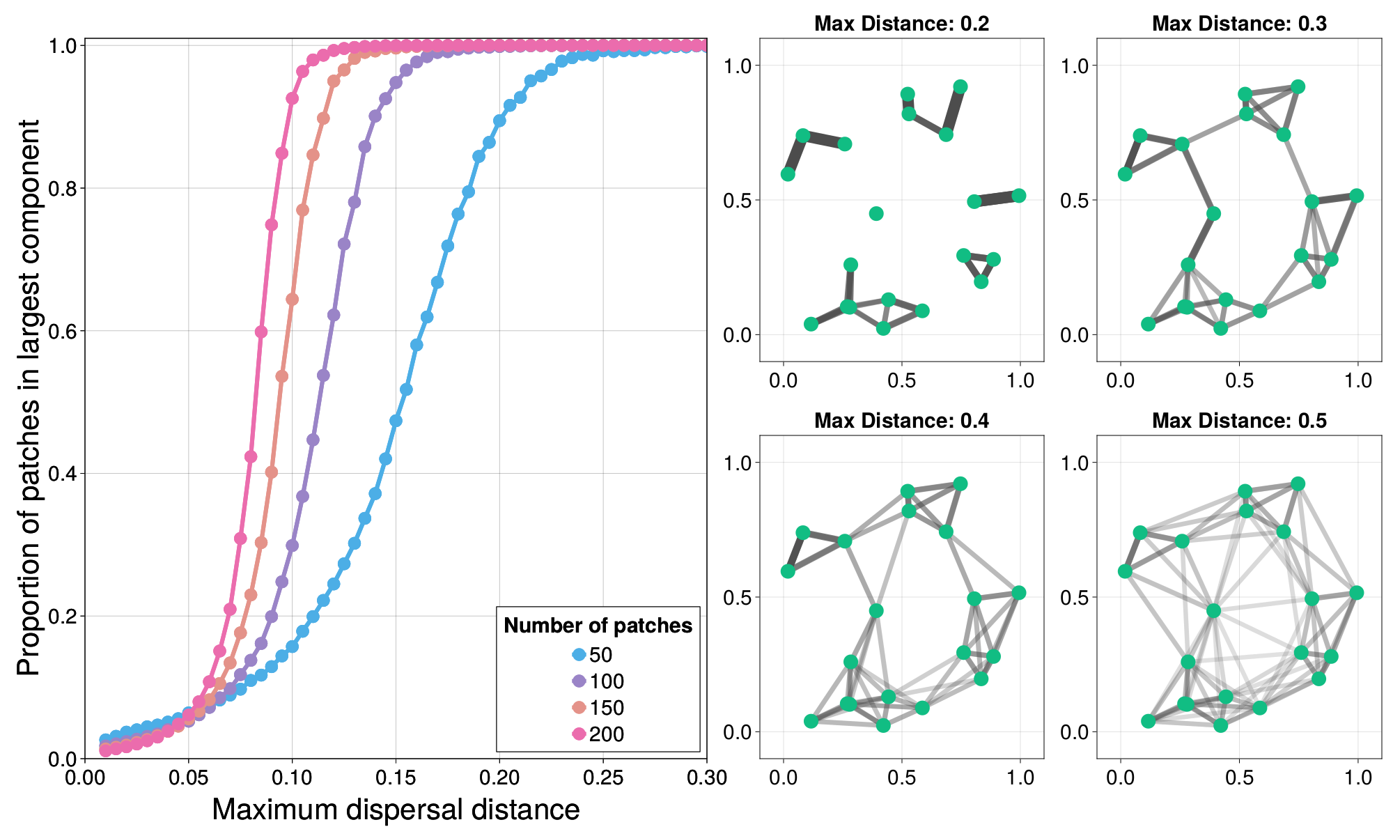
Phase transitions in the percolation of habitat connectivity

We begin by examining the effect of maximum dispersal distance, a trait with important consequences for home and total range size [@Bowman2002DisDis; @Whitmee2013PreDis], on landscape connectivity, and demonstrate a sudden phase-transition in the connectivity patchy landscapes. In the real world, there are intrinsic biological constraints that make dispersal beyond a certain distance effectively impossible. As the maximum dispersal distance of the species in question changes, so does the topology of the resulting spatial graph, depending on how many patches there are and where they are located, this means that there are patches that are entirely isolated, or small “meso-populations” that interact with a few other patches, but not the larger system as a whole (figure 3).

A classic result in network science is the phase transition associated with the emergence of a “giant-component” in random Erdos-Renyi graphs [@Erdos1959RanGra; @Newman2018Net]. In this case, a “giant-component” refers to a set of at least half the nodes in the network that are connected via some path. A similar phase transition occurs here as we increase the maximum dispersal distance of a hypothetical species. In Figure @fig:percolation (left), we see the proportion of patches that are connected via some path ("in the largest component”) as a function of maximum dispersal distance, and find that this transitions becomes increasingly critical as the number of patches increases---meaning the jump from almost no patches being connected to nearly all being connected occurs increasingly rapidly as soon as a critical threshold of maximum dispersal distance has been reached.

Each point in Figure @fig:percolation represents 512 random spatial graphs generated at that given maximum dispersal distance. A single instance can be run with

function run_instance(num_patches, max_dispersal_distance)
	dk = DispersalKernel(max_distance=max_dispersal_distance)
	sg = SpatialGraph(Coordinates(num_patches), dk)
	g = Graph(sg.potential .> 0)
	component_sizes = length.(Graphs.connected_components(g))
	return maximum(component_sizes)
end

which computes the size of the largest component of the spatial graph using the Graphs.jl package.

{#fig:percolation}

Measuring the spatial inflationary effect as a function of dispersal distance

A well-known phenomenon in patchy landscapes is that the inherent variation in habitat patch quality can lead to some patches acting as “sources”, where the intrinsic growth rate of a population is positive, and “sinks”, where the growth rate is negative [@Pulliam1988SouSin]. The balance of both sources and sinks determines the persistence of a metapopulation in a patchy landscape, though this may not be as simple as a majority-rule decision. Here we demonstrate that landscape connectivity plays a crucial role in determining whether there is a “colonization-credit” [@Cristofoli2010ColCre] that enables the metapopulation to persist, despite a minority of patches having positive growth rate. This effect has been documented in a large number of systems [@Bagaria2015AssCoe; @Duplisea2016ExtDeb; @Haddou2022WidExt; @Rumpf2019ExtDeb] and is likely to be important to predict which species will be capable of tracking their climatic niche over the coming century [@Talluto2017ExtDeb].

If the environmental conditions that give rise to “source” or “sink” behavior are spatially autocorrelated, there may be a similar spatial analogue to the inflationary effect [@Gonzalez2002InfEff]---where temporal autocorrelation in environmental conditions can cause “sink” patches to have greater expected abundance than if the patch experiences a constant environment [@Matthews2007InfEff; @Roy2005TemAut].

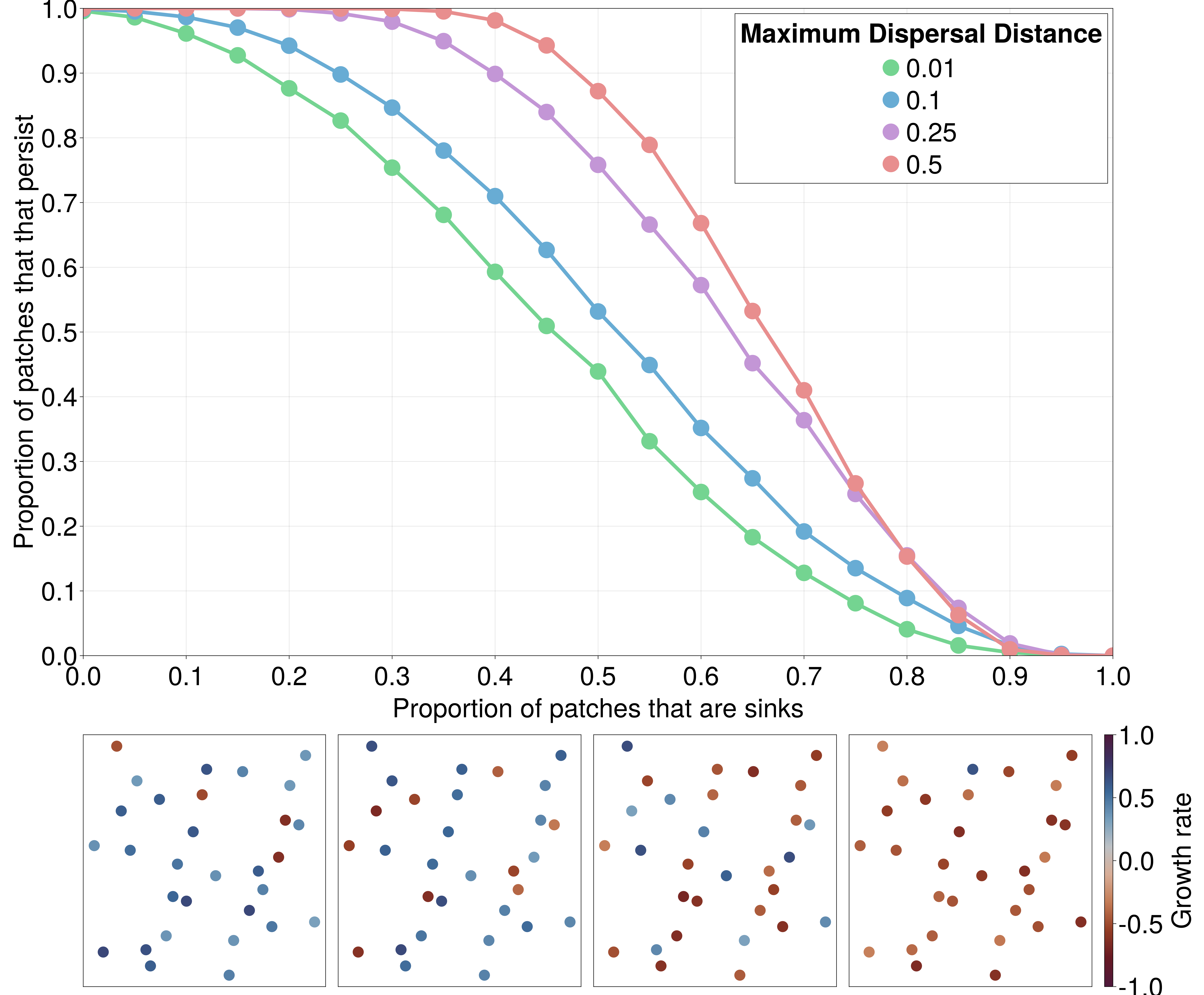
To demonstrate this using EcoDynamics.jl, we simulate the Beverton-Holt model (a stochastic, discrete-time model of population dynamics) for 250 generations across spatial graphs with a fixed ratio of sources:sinks. We simulate 512 random spatial graphs, each with 50 patches, at each value of the proportion of patches that are sinks, ranging from 0 to 1 (Figure 4). This vignette highlights the integration between NeutralLandscapes.jl and EcoDynamics.jl, creating spatial graphs with autocorrelated environmental conditions using the following:

function make_graph(max_dispersal_distance)
    el = EnvironmentLayer(generator=MidpointDisplacement(0.8)) 
    coords = Coordinates(el)
    sg = SpatialGraph(coords, DispersalKernel(max_distance=max_dispersal_distance)) 
end

This provides a spatial graph with an environmental covariate associated between 0 and 1 with each patch (called x by default). The underlying environmental variable is generated using the `MidpointDisplacement`` neutral landscape generator from NeutralLandscapes.jl, and takes $H = 0.8$ as a parameter controlling spatial autocorrelation.

To relate this environmental covariate to the dynamics that occur in each patch, we define a niche function

function niche(model, traits, local_env)
    θ = paramdict(model)
    θ[:R₀] = (cutoff - local_env[:x])
    return θ
end

We find that as the maximum dispersal distance (colors in Figure 4) increases, the proportion of patches that are able to persist when exactly half of the patches are sinks (and the other half are sources; 0.5 on the horizontal axis of Figure 4), the “surplus” number of patches above half that are able to persist, despite having negative growth rate, increases.

{#fig:inflation}

Bayesian Inference of Consumer-Resource Dynamics

The second pair of case studies deal with scenarios where we have a time-series of observed dynamics, which are potentially quite sparse in time and subject to lots of measurement error. In this case, we are solving the inverse problem [@Stouffer2019AllEco]---going from a set of observations to inference about the parameters underlying the generating process. In both examples, we will deal with the dynamics of a Rosenzweig-MacArthur (RM) consumer-resource model, given by the equations

\begin{align*} \frac{dR}{dt} &= \lambda R \bigg(1 - \frac{R}{K} \bigg) - \frac{\alpha CR }{1-\alpha \eta R} \ \frac{dC}{dt} &= \beta \frac{\alpha CR}{1-\alpha \eta R} - \gamma C \end{align*}

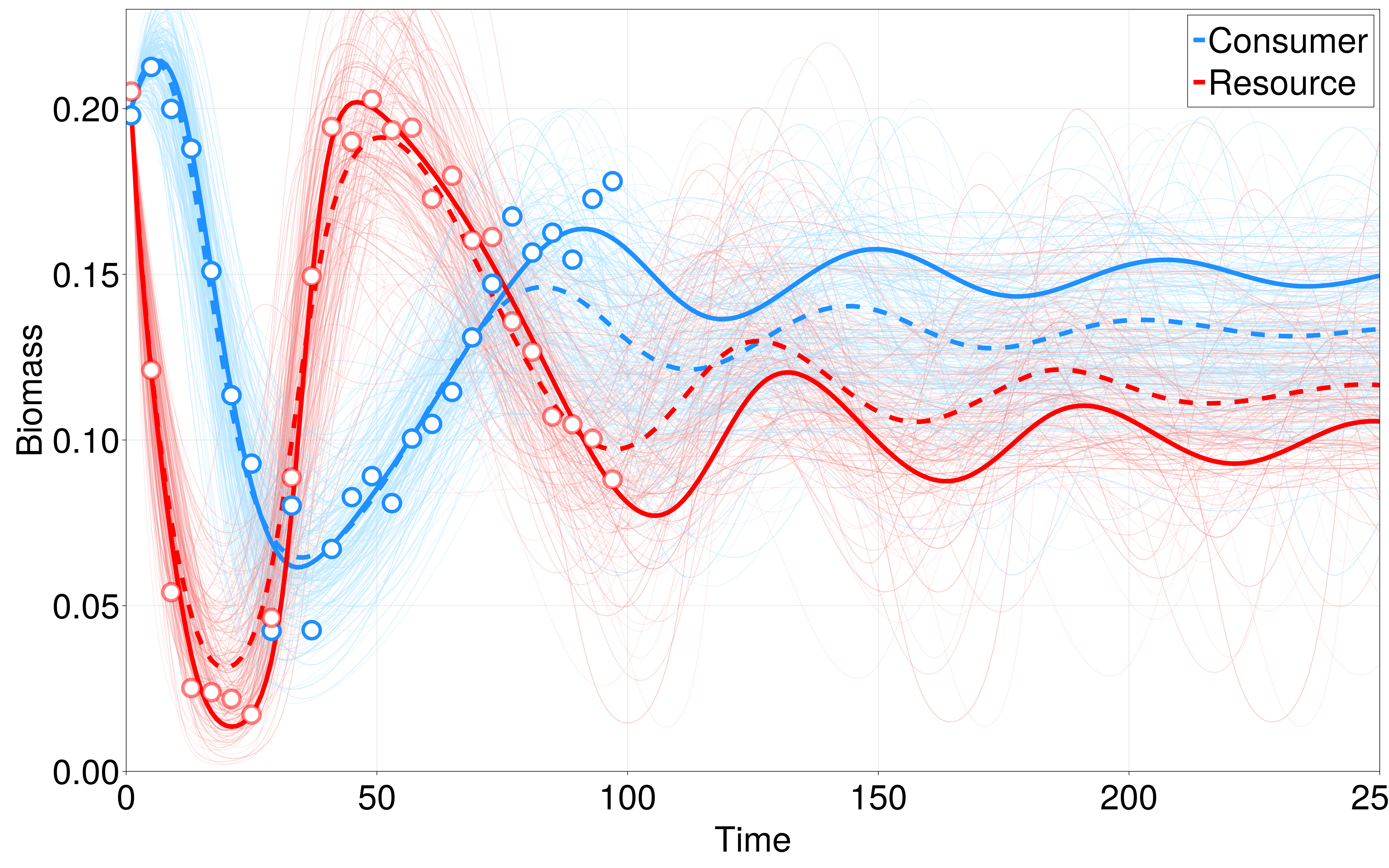
Note that this is effectively resource logistic growth with consumption given by a Holling Type-II functional response. The RM system is particularly well studied as it undergoes a Hopf-bifurcation as the value of $K$ increases (Roos 2023; Rosenzweig 1971), moving from a place where both abundances approach a stable spiral fixed point, to a point with permanently oscillating limit cycles. As K continues to increase beyond the Hopf bifurcation point, the amplitude of the oscillations for both species increases---in real systems this destabilizes dynamics as the increasing amplitude of each species’ oscillations means points in the trajectory get closer and closer to extinction (zero abundance), and as a result this system is often cited as defining the “paradox of enrichment”.

We infer the parameters of this system using a simple interface from EcoDynamics.jl to to Turing.jl, a Julia library for Bayesian inference and probabilistic programming (Note that there are also interfaces to STAN using DiffEqBayes.jl or STAN.jl). The results of this inference are shown in Figure @fig:bayes_inference. Note that although this is fairly effective at learning the true parameters and resulting dynamics from sparse, noisy data, this comes with a large modeling trade-off, which is that we must a priori specify that we believe that the underlying dynamics follow the Rosenzweig-MacArthur form. We are, of course, free to fit this data to a wide-variety of functional forms of consumer-resource dynamics and apply model selection techniques (e.g. AIC, MDL) to select which form most effectively describes our data, though the scalability of this approach begins to break down when confronted with larger food-webs with potentially heterogeneous functional responses between different species.

{#fig:bayes_inference}

Accounting for “missing-ecology” using ecology-informed neural networks

Scientific Machine Learning and Physics Informed Neural Networks

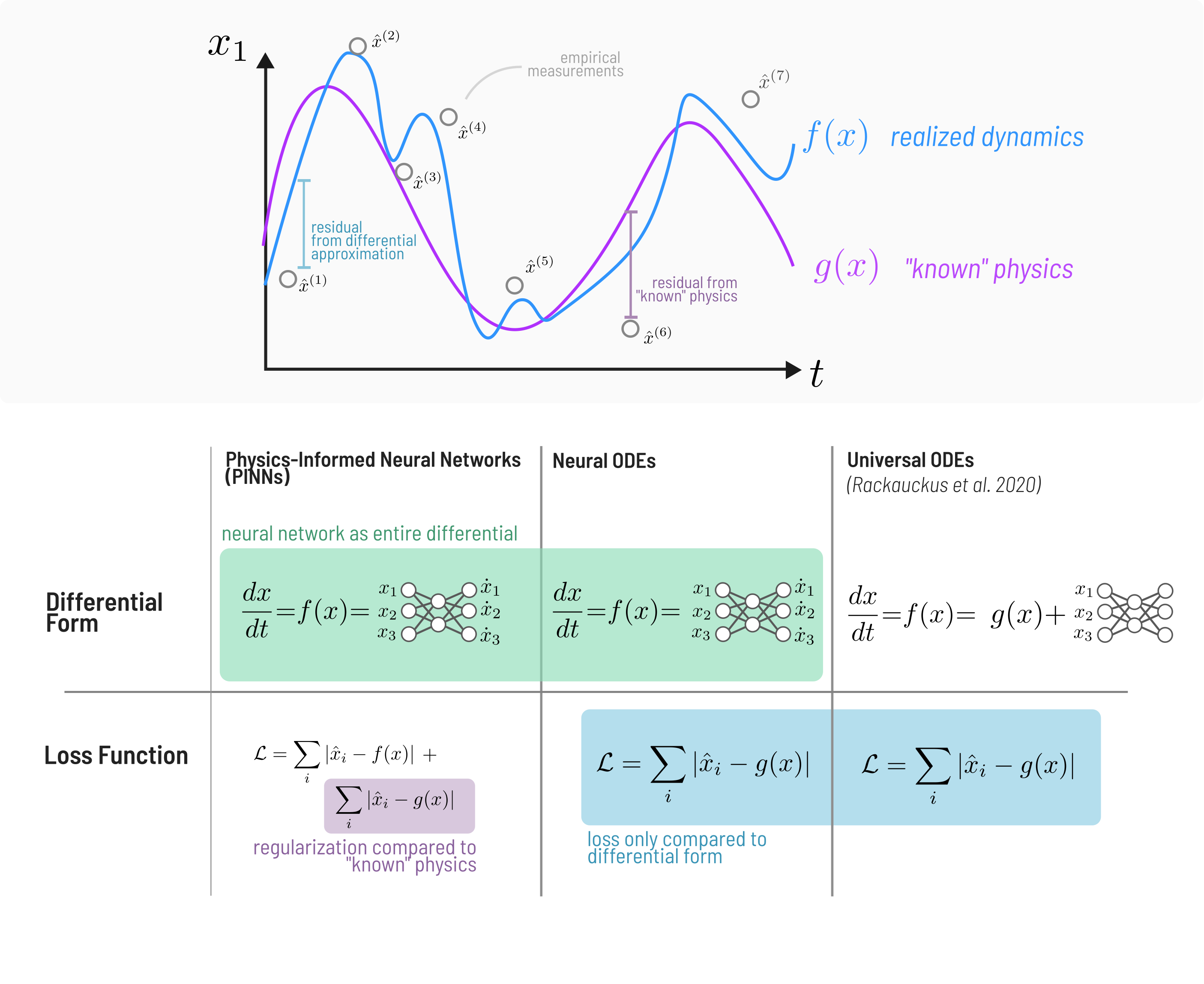
In many complex systems, and ecology especially, the true form of the underlying dynamics are not fully known. This problem has led to novel approaches that integrate machine learning with conventional differential equation models of systems to capture “unknown” or “missing” parts of the models. Specifically in fluid-dynamics, this practice has led to much research interest in statistical methods for accounting for the inherent sparsity of data in many high-dimensional non-linear systems and learning efficient representations of their dynamics [@Brunton2016DisGov]---the general approach being to find a coordinate basis that enables simpler representation of the underlying dynamics than in a Cartesian basis. Moving beyond typical statistical approaches to accomplish this same goal, Physics-Informed-Neural-Networks (PINNs) are used to combine mechanistic physical models with neural networks. This research has led to development of many similar but distinct models---both Neural ODEs (NODEs, @Chen2018NeuOrd, @Dandekar2022BayNeu) and Universal ODEs (UODEs; @Rackauckas2021UniDif).

A brief summary of the differences is shown in Figure 4. The primary differences are that PINNs include distance from the prediction of a physical law directly in the loss function, which neither NODEs nor UODEs do. Both PINNs and NODEs use a neural network to approximate the entire differential ($\frac{dx}{dt}= \text{NN}(x)$), where the loss function only considers the distance from the data, while, UODEs only approximate the residual between “known” dynamics and data, i.e. $\frac{dx}{dt}=g(x) + \text{NN}(x)$, where $g$ is what is known a priori about the equations governing the dynamics of the system. Note that UODEs are a superset of NODEs, as setting the $g(x)$ term in a UODE to $0$ results in a standard NODE (technically the formalism of UODEs makes them a superset of any stochastic delay partial differential equation, though the details are out of scope for this paper, see @Rackauckas2021UniDif for more information).

Julia has one of the most mature ecosystems for SciML, enabling straightforward interfaces from the various software packages for SciML (DataDrivenDiffEq.jl, DiffEqFlux.jl, SymbolicRegression.jl, etc.) to EcoDynamics.jl.

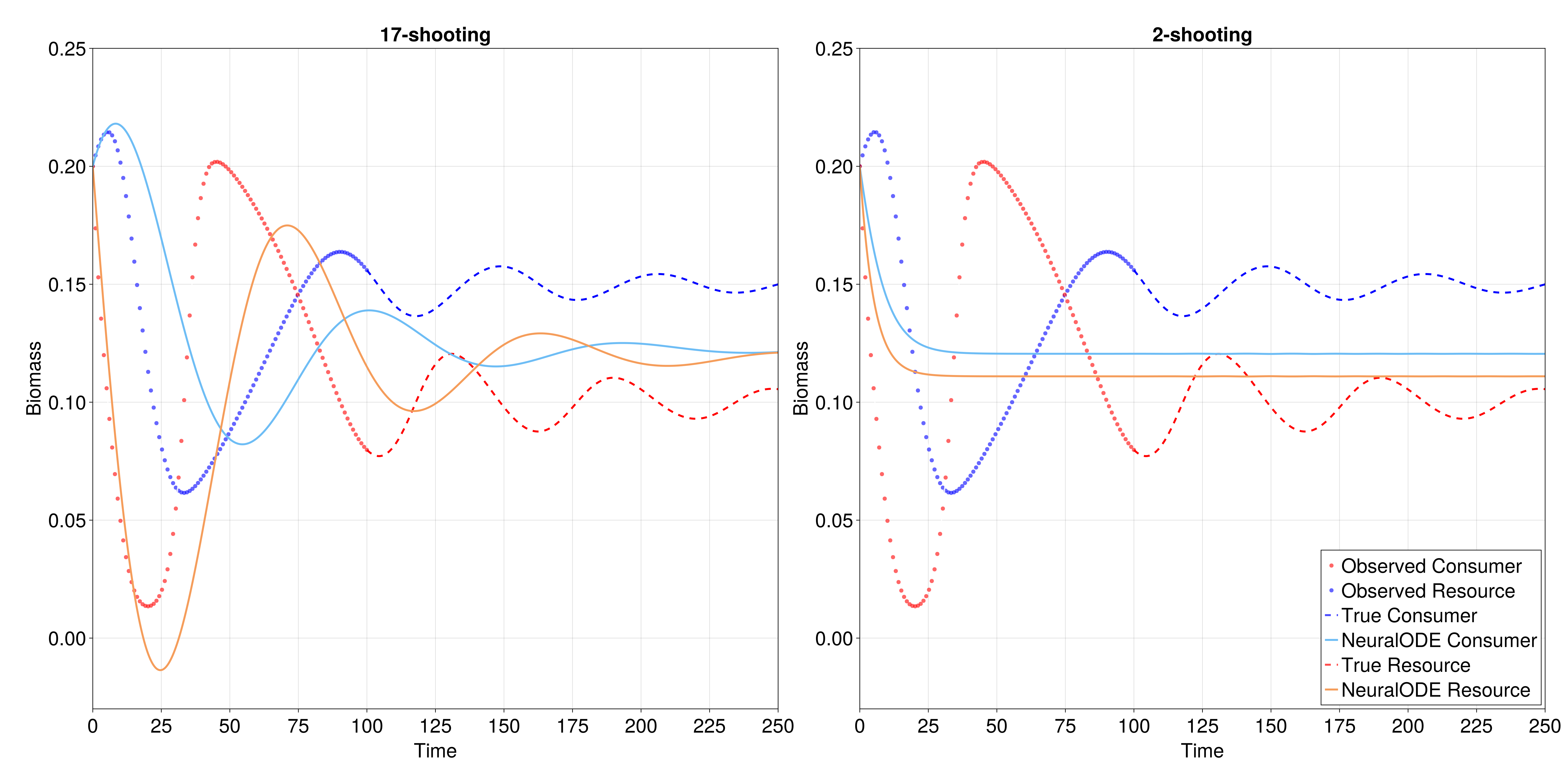
Inferring a functional response using Ecology Informed Neural Networks

In this vignette, we demonstrate the integration between EcoDynamics.jl and the Julia SciML ecosystem to fit a NeuralODE to data from the Rosenzweig-MacArthur model. We demonstrate a result from @Boussange2022MinEco, which is that capturing nonlinear dynamics using NeuralODEs is much easier when training NODEs using a method called “multiple-shooting” (also referred to as “mini-batching”; @Turan2022MulSho).

The default perspective when training a NODE on a time-series is to compute a single loss value across all pairs of adjacent time-points,

$$\mathcal{L} = \sum_{t \in {2\dots N_t}} |x_{t-1} - \hat{x}_t|$$

though this tends to undefit oscillatory dynamics [@Turan2022MulSho], which are particularly common in ecological models. To address this, multiple shooting fits the loss function by splitting the original time-series into many smaller, shorter time-series, and evaluates the loss as a combination the sum of the loss across all unique segments, and a separate term that evaluates the distance between the end point of each segment and the start of the next one.

{#fig:sciml}

Discussion

Here we have showcased EcoDynamics.jl, a software package for population and community dynamics on spatial graphs in the Julia language. This software package includes a library of common models for both occupancy and abundance dynamics, and an interface to easily add custom models. Further, EcoDynamics.jl enables species traits and heterogeneous environmental conditions across patches to influence dynamics, and includes methods for simulating observation error to generate synthetic datasets for benchmarking and validation of models for inference from time-series data. This is all built on top of DifferentialEquations.jl, a state-of-the-art library for simulation of deterministic and stochastic differential equations [@Rackauckas2017DifJl]. The aim of this toolkit is to standardize methods for generating synthetic data, and to serve as a “virtual laboratory” [@Grimm2005IndMod] for testing sampling designs and inference tools in silico.

The metacommunity concept has demonstrated its utility in scaling from local community processes to describe the distribution and abundance of species across space and time [@Leibold2004MetCon; @Leibold2017MetEco]. Metacommunity theory is built around understanding the composition of species across heterogeneous landscapes by treating them as networks of networks [@Hutchinson2019SeeFor]. A standardized toolkit for community dynamics on spatial graphs is needed to better understand these systems, with the ability to rapidly prototype “virtual experiments”, and to produce phase-diagrams of the metacommunity paradigm (species-sorting, patch dynamics, mass effect, neutral; @Leibold2004MetCon) that result from the balance of the fundamental mechanisms that govern community ecology [@Vellend2010ConSyn]. A downstream requirement for this software to enable virtual experiments potentially involving spatial heterogeneity, environmental perturbation, interspecific variation in response to the environment, and so on, is that this toolkit must be both flexible enough to enable custom extension, but also fast enough to scale to large-scale batch simulation.

We hope this is the foundation of developing a robust, standardized set of tools for ecological dynamics in the Julia language. There is increased interest in developing a “digital twin” for biodiversity [@Koning2023DigTwi], and it is increasingly accepted that we will not be able to detect and attribute the causes of biodiversity without sufficient monitoring and modeling tools [@Gonzalez2023FraDet].

We have also demonstrated the potential utility of Scientific Machine Learning (SciML;@Rackauckas2021UniDif) for learning complex ecological dynamics from limited training data. Despite a wide variety of theoretical and applied advances being made in this field over the last decade, its adoption in ecology is slow, despite its potential [@Boussange2022MinEco; @Chen2019RevCom]. The ability to mix mechanistic models with data-driven methods from machine learning offers particular advantages in ecology, where there is often considerable variation in data, even given a shared mechanism, due to the inherent stochasticity of many ecological processes.

EcoDynamics.jl is built on two approximations: the spatial graph approximation of patchy landscapes, and the reaction-diffusion approximation of dispersal. These abstractions, like all abstractions in ecological modeling, are only valid for a particular set of scales. One possible use of EcoDynamics.jl is to validate these assumptions in comparison to simulation models designed around smaller scales to determine when and why these approximations break down. For example, diffusion may be an adequate approximation for dispersal if it is a stationary process, but if the dispersal distribution is characterized by rare events (i.e the distribution kernel is fat-tailed), then using the expected value of that process at each timestep (as diffusion does) may not be a valid assumption at all. Similarly, the spatial-graph assumption makes strong assumptions about the quality of habitat that is not a core patch---namely that it is inhospitable.

Such models may not adequately represent that movement process of many organisms, but determining when this approximation is valid is essential to know when it is useful for making predictions and decisions in a conservation or management context. It is worth remembering that as scientists, we make approximations for a reason. When considering something as complex as an ecosystem, it can become tempting to imagine that the ontological validity only lies in the smallest scales, and that each approximation moves us further and further from ecological reality. Yet it is obvious that basing ecological models on the smallest scales possible is both computationally intensive enough to be impractical, and also unlikely to provide as much insight as it creates nearly as many problems as it solves---“Abstraction becomes destructive when the abstract is reified and when the historical process of abstraction is forgotten, so that the abstract descriptions are taken for descriptions of the actual objects...The problem for science is to understand the proper domain of explanation of each abstraction rather than become its prisoner” [@Levins1987DiaBio].

We conclude by reemphasizing the need for tools like EcoDynamics.jl to simulate synthetic data for the purpose of testing and validating methods for inference from data before they encounter data for which the true generating process is unknown. Ecologists, and all other sciences, inevitably are faced with the task of drawing inference from data that they wish they knew much more about. Real data will always be shrouded in the uncertainty that we are unsure what the true process(es) generating the data is, and that we can not be certain about how biased our measurements are. By using mechanistic models to simulate many “possible worlds”, we can at least benchmark and validate the methods we use for inference and get a reasonable expectation of the predictive efficacy of our forecasts. This is essential if we are to produce forecasts that are not only robust, but adequately reflect the uncertainty in their predictions [@Urban2016ImpFor].

gottacatchenall/ms_ecodynamics_jl