A repository for the ICLR 2023 paper Information-Theoretic Diffusion containing simplified code and examples. The paper introduces an exact equivalence between probability and optimal denoising. Mathematically, this is expressed as,
where
@inproceedings{
kong2023informationtheoretic,
title={Information-Theoretic Diffusion},
author={Xianghao Kong and Rob Brekelmans and Greg {Ver Steeg}},
booktitle={International Conference on Learning Representations},
year={2023},
url={https://arxiv.org/abs/2302.03792} }
To install requirements:
pip install numpy scipy matplotlib scikit-learn torch torchvision pytorch-lightning tensorboard diffusers
This repository is simplified compared to the main repository:
- Only consider continuous density estimation (most diffusion papers treat pixels as discrete)
- Omits the ensembling which improves results but complicates the code
- Treats the log-logistic distribution (location, scale) as hyper-parameters (see below), rather than estimating them as done in the paper.
- Pytorch lightning is used to simplify boilerplate, and makes it easier to exploit different compute resources.
To train and generate figures, run this script.
python train_2d.py --dataset {dino,moons,scg,line,circle}
Run with --help flag to see hyper-parameters.
Statistics and image outputs appear in tensorboard.
tensorboard --logdir .
The main ideas can be read in the class in diffusionmodel.py. The diffusion model takes a denoising architecture as input (arguments are input and log SNR, output has the same size of input). This simplified code assumes continuous density estimation, and requires specifying the log SNR range (see discussion below).
The main repository contains the paper code including CIFAR-10 experiments. The following command trains a CIFAR-10 model using IT diffusion, starting with a pretrained U-Net. See --help for more options, including training from scratch.
python train_cifar10.py
MSE curves and log likelihoods are tracked in tensorboard. Checkpoints are saved automatically by Pytorch Lightning.
This is the equivalent step to fixing the noise scheduler in other diffusion papers. In our paper, we found that the logistic distribution over log SNR values is optimal for Gaussians and a good choice for more complex distributions like CIFAR. We only need to estimate two parameters, the location and scale of this distribution. In the paper, we estimate them from the spectrum of the data.
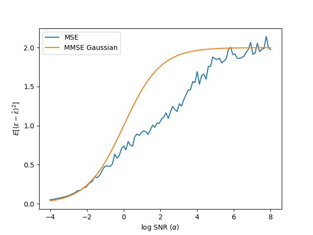
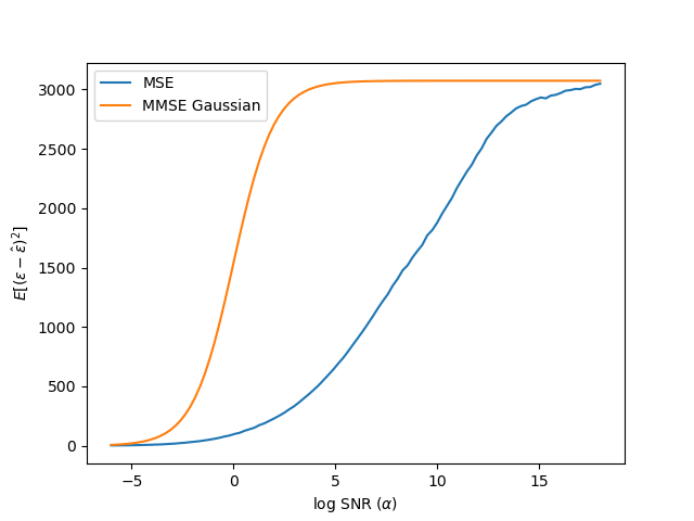
However, it may be simpler to estimate these parameters directly by looking at the MSE curves. To empirically set these hyper-parameters, run the diffusion model once with the default values, and then use tensorboard to look at the MSE plot.
Ideally, you'd set the location, logsnr_loc to be the 50 percent quantile, and the scale to be the distance from the 50 percent quantile to the 25th or 75th percent quantile. (Note the maximum value for MSE should be d, so you should divide by d to interpret these as quantiles.) More heuristically, you want the location to be in the middle of the gap between the MMSE Gaussian curve, and the true MSE curve. This is also a good way to diagnose training, as we should always do at least as well as the Gaussian MMSE. Note that the MSE curve (shown for epsilon) is not necessarily monotonic. If the data is exactly on a low-d manifold (like the dino line drawing), the MSEs can go to zero at high log SNR. The same is true for discrete data, as shown in the paper. In these cases, the differential entropy is formally negative infinite. We get an upper bound from cutting off our log SNR at finite values (and from not necessarily finding the true MMSE).
We visualize the density as contour plots using
The strongly correlated Gaussian is a nice test case. We know the true entropy (1.22 nats) and can check
that our validation loss approaches this number.

A fun, highly nonlinear density, that is strongly peaked on a low-dimensional manifold.
A classic example - we can see that we have a low density (white) area that splits the two clusters.

Uniform disribution in a square. The sharp edges are not well modeled by samplers but seem to be captured well by the probability density.
For location and scale of the logistic importance sampling distribution, we used (6, 3). The MSE curve after 50 epochs of training is shown below.
The validation loss is about -8400 nats. Converting to bits/dim, we would get -8400 / log(2) / (32323) = -3.94. This result is comparable to the result "DDPM-tuned" in the paper Table 1, and is almost identical despite the simplifications to the method.
Inspired by the tiny diffusion repo. To reproduce results in the paper, see our main repository.


