| Documentation |
|---|
  |
| Build Status |
| Community |
| Acknowledgement |
The visualization of numerical results is an important part of finite element (FE) computations. However, before the inception of GridapMakie.jl, the only approach available to data visualization of Gridap.jl computations was to write simulation data to data files (e.g., in vtu format) for later visualization with, e.g., Paraview or VisIt. From the idea of visually inspecting data from Julia code directly or to manipulate it with packages of the Julia open-source package ecosystem, GridapMakie.jl is born. As a part of the Google Summer of Code 2021 program, GridapMakie adopts Makie.jl as a second visualization back-end for Gridap.jl simulations. This package is thought as a built-in tool to assess the user in their FE calculations with a smoother workflow in a highly intuitive API.
A significant part of this package has been developed in the framework of the Google Summer of Code 2021 project [Gridap] Visualizing PDE approximations in Julia with Gridap.jl and Makie.jl.
According to Makie's guidelines, it is enough to install one of its backends, e.g. GLMakie. Additionally, Gridap provides the plot objects
to be visualized and FileIO allows to save the figures plotted.
julia> ]
pkg> add Gridap, GridapMakie, GLMakie, FileIOFirst things first, we shall be using the three packages as well as FileIO.
We may as well create directories to store downloaded meshes and output files
using Gridap, GridapMakie, GLMakie
using FileIO
mkdir("models")
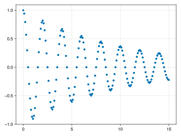
mkdir("images")Let us consider a 1D triangulation Ω, a function u and the corresponding FE function uh constructed with Gridap
model = CartesianDiscreteModel((0,15),150)
Ω = Triangulation(model)
reffe = ReferenceFE(lagrangian, Float64, 1)
V = FESpace(model, reffe)
u=x->cos(π*x[1])*exp(-x[1]/10)
uh = interpolate(u, V)
The visualization of the function can be achieved as follows
fig=plot(uh)
save("images/1d_Fig1.png", fig)
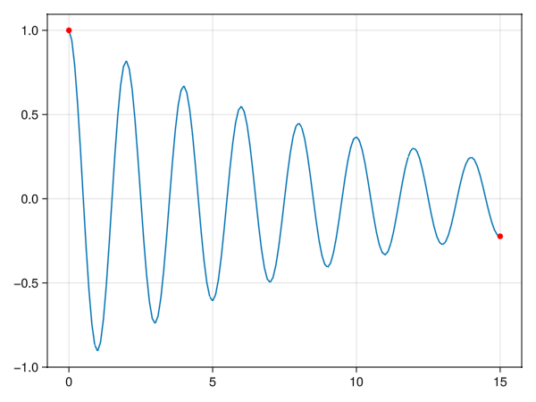
We may also plot the function with a line and its value at the boundaries
Γ = BoundaryTriangulation(model)
fig=lines(Ω,u)
plot!(Γ,uh,color=:red)
save("images/1d_Fig2.png", fig)Then, let us consider a simple, 2D simplexified cartesian triangulation Ω
domain = (0, 1, 0, 1)
cell_nums = (10, 10)
model = CartesianDiscreteModel(domain, cell_nums) |> simplexify
Ω = Triangulation(model)
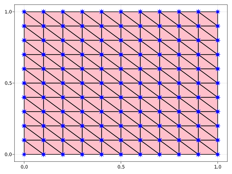
The visualization of the vertices, edges, and faces of Ω can be achieved as follows
fig = plot(Ω)
wireframe!(Ω, color=:black, linewidth=2)
scatter!(Ω, marker=:star8, markersize=20, color=:blue)
save("images/2d_Fig1.png", fig)
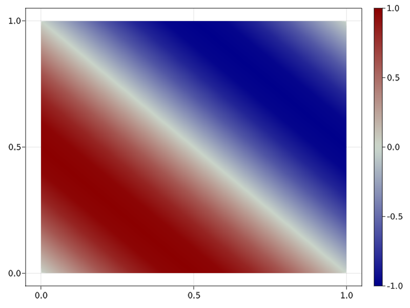
We now consider a FE function uh constructed with Gridap
reffe = ReferenceFE(lagrangian, Float64, 1)
V = FESpace(model, reffe)
uh = interpolate(x->sin(π*(x[1]+x[2])), V)
and plot it over Ω, adding a colorbar
fig, _ , plt = plot(Ω, uh)
Colorbar(fig[1,2], plt)
save("images/2d_Fig11.png", fig)
On the other hand, we may as well plot cell values
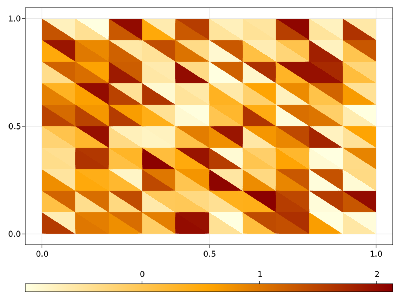
celldata = π*rand(num_cells(Ω)) .-1
fig, _ , plt = plot(Ω, color=celldata, colormap=:heat)
Colorbar(fig[2,1], plt, vertical=false)
save("images/2d_Fig13.png", fig)
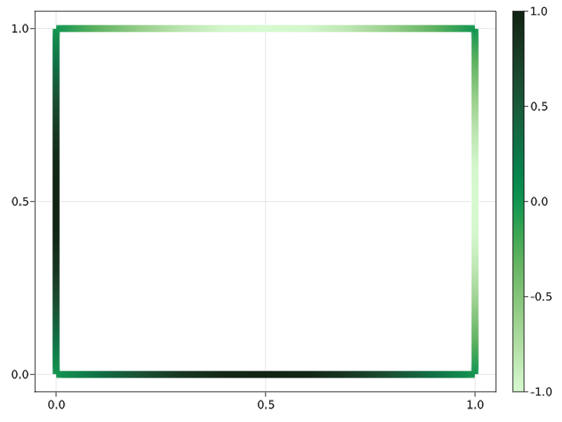
If we are only interested in the boundary of Ω, namely Γ
Γ = BoundaryTriangulation(model)
fig, _ , plt = plot(Γ, uh, colormap=:algae, linewidth=10)
Colorbar(fig[1,2], plt)
save("images/2d_Fig111.png", fig)In addition to the 2D plots, GridapMakie is able to handle more complex geometries. For example, take the mesh from the first Gridap tutorial, which can be downloaded using
url = "https://github.com/gridap/GridapMakie.jl/raw/d5d74190e68bd310483fead8a4154235a61815c5/_readme/model.json"
download(url,"models/model.json")
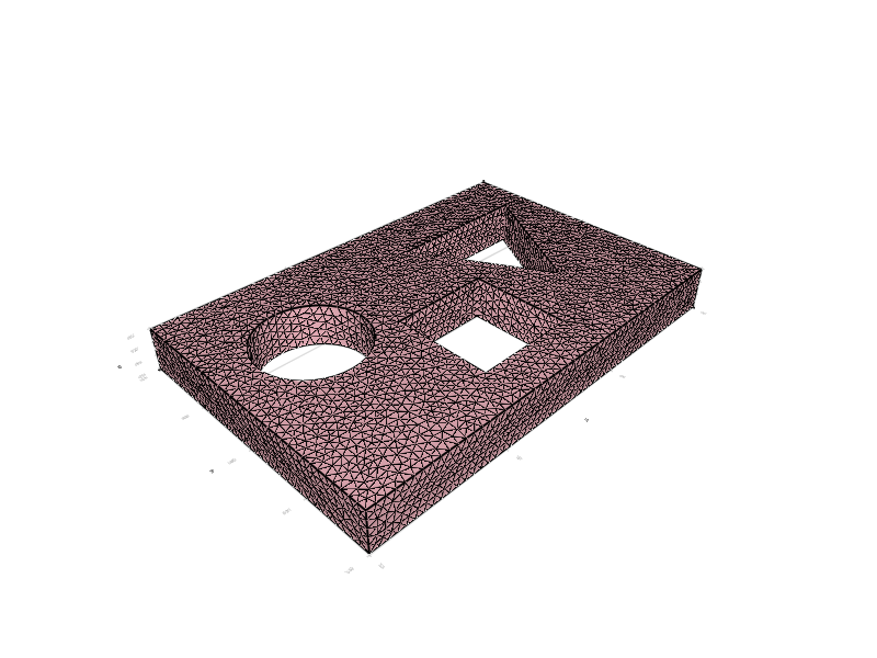
Therefore, we may as well visualize such mesh
model = DiscreteModelFromFile("models/model.json")
Ω = Triangulation(model)
∂Ω = BoundaryTriangulation(model)
fig = plot(Ω)
wireframe!(∂Ω, color=:black)
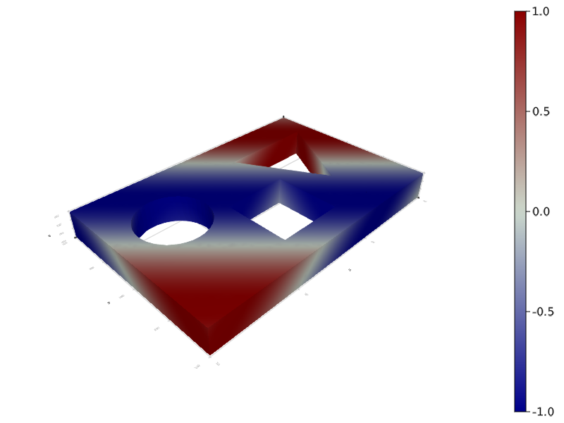
save("images/3d_Fig1.png", fig)v(x) = sin(π*(x[1]+x[2]+x[3]))
fig, ax, plt = plot(Ω, v)
Colorbar(fig[1,2], plt)
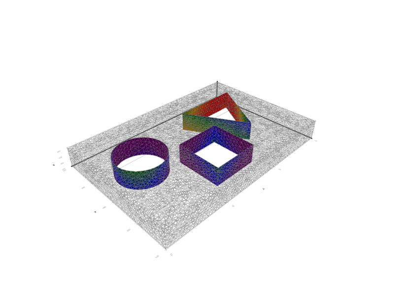
save("images/3d_Fig2.png", fig)we can even plot functions in certain subdomains, e.g.
Γ = BoundaryTriangulation(model, tags=["square", "triangle", "circle"])
fig = plot(Γ, v, colormap=:rainbow)
wireframe!(∂Ω, linewidth=0.5, color=:gray)
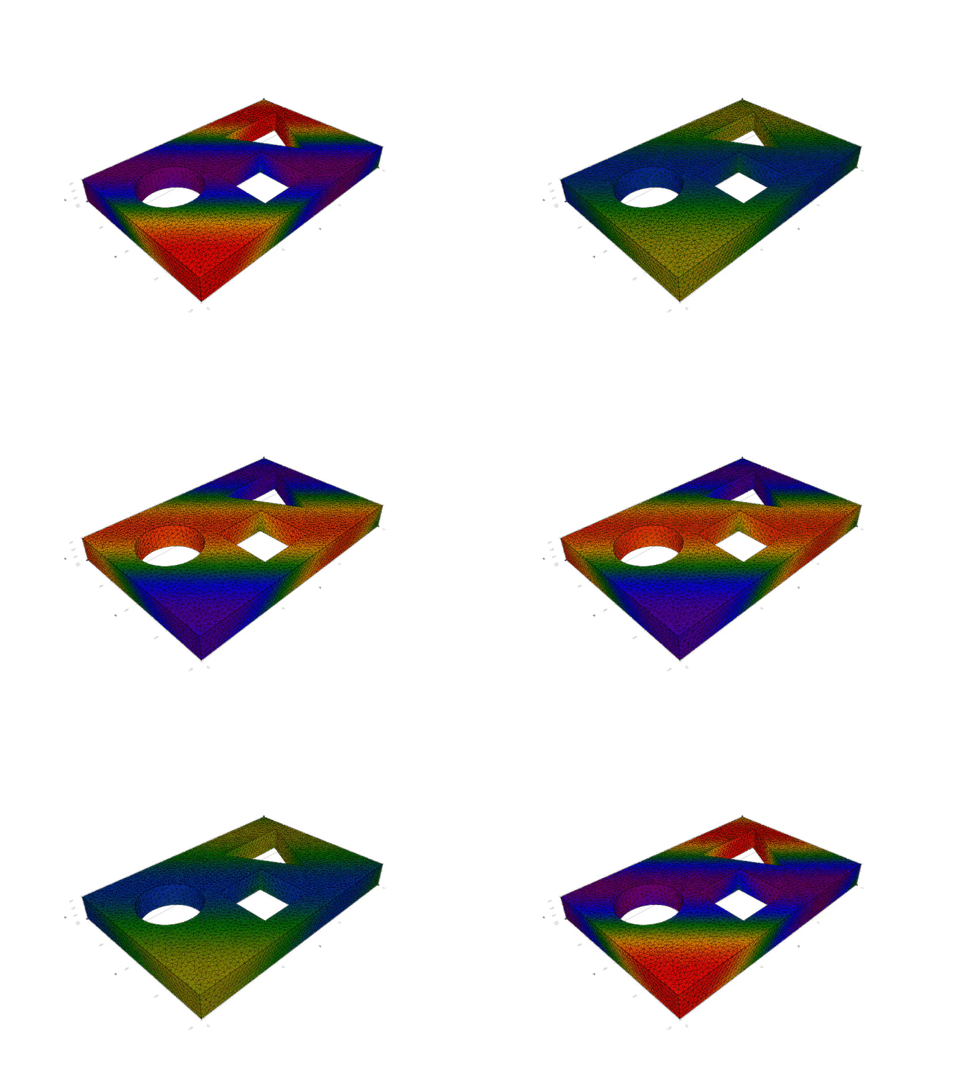
save("images/3d_Fig3.png", fig)Finally, by using Makie Observables, we can create animations or interactive plots. For example, if the nodal field has a time dependence
t = Observable(0.0)
u = lift(t) do t
    x->sin(π*(x[1]+x[2]+x[3]))*cos(π*t)
end
fig = plot(Ω, u, colormap=:rainbow, colorrange=(-1,1))
wireframe!(∂Ω, color=:black, linewidth=0.5)
framerate = 30
timestamps = range(0, 2, step=1/framerate)
record(fig, "images/animation.gif", timestamps; framerate=framerate) do this_t
    t[] = this_t
end
This page was generated using Literate.jl.
