MixEntroPY

Numpy & PyTorch vectorized implementation of various differential entropy estimators for ML & DL.

About The Project

Information theory-inspired machine learning methods are gaining increasing interest, with estimation of the entropy as well as mutual information of random variables serving as their cornerstone.

To estimate the Shannon entropy of a discrete random variable, given its probability distribution, one can simply apply the definition of Shannon entropy $H(x)=-\sum_i p(x_i)\log p(x_i)$ to obtain an accurate result.

But when it comes to estimate differential entropy, $h(x)=-\int p(x)\log p(x)dx$, from data points sampled from datasets or models, often there is no prior knowledge about the underlying distribution.

In such cases, we could make an assumption of the unknown distribution and expect the assumed distribution to have a closed-form expression for its entropy calculation, e.g., multivariate Gaussian.

Kernel Density Estimation(KDE) is one of commonly used methods to approximate probability density of a distribution, However, while a single kernel may have a closed-form expression for its entropy, the mixture of these kernels typically does not.

This project offers several entropy estimators for these mixture distributions, (mainly focus on mixture of Gaussian and mixture of uniform), implemented with both Numpy and PyTorch.

Most of the estimators are differentiable, making them suitable for optimization purposes.

Getting Started

Installation

Switch to your desired virtual/conda env with python >= 3.8:

To install with numpy dependency only:
pip install mixentropy

To install with both numpy and pytorch dependency:
pip install mixentropy[pth]

(Optional) In order to run experiments, you may also need:
pip install matplotlib scipy

Usage

Estimators for mixture distribution takes:

c: Weights of each components, which should sum up to one;
mu: Positions of each component.
- For Gaussian, mu indicates mean of each component;
- For uniform, mu indicates center position of each component.
sigma: "Spread" of each component.
- For Gaussian, sigma is a stack of variance (or covariance matrix for multivariate Gaussian) of each component,
- For uniform, sigma is a stack of diagonal matrices, with each diagonal entry indicates interval length of a component on that dimension.
elem: component type, could be "gauss" or "uniform", for Gaussian and uniform respectively.

Some estimator may take extra arguments:

Monte Carlo estimator needs n_samples to indicate how many datapoints will be sampled to estimate entropy.
Pairwise distance estimator needs dist to indicate which distance function to use (could be "kl" or "chernoff").

Example

import numpy as np
import torch
from mixentropy.np.monte_carlo_estimator import estimate as h_mc_np
from mixentropy.np.kde_estimator import estimate as h_kde_np
from mixentropy.np.elk_estimator import estimate as h_elk_np
from mixentropy.np.pairwise_dist_estimator import estimate as h_pairwise_np
from mixentropy.pth.monte_carlo_estimator import estimate as h_mc_pt
from mixentropy.pth.kde_estimator import estimate as h_kde_pt
from mixentropy.pth.elk_estimator import estimate as h_elk_pt
from mixentropy.pth.pairwise_dist_estimator import estimate as h_pairwise_pt


# generate some random fake data
k = 100  # number of components
d = 10  # number of dimensions of each component
b = 4  # batch size
c = np.ones(k) / k  # [k,], weights for k components
mu = np.random.normal(0., 1, size=(k, d))  # [k, d], n components, each has d dimensions
sigma = np.stack([np.eye(d)] * k)  # [k, d, d], k components, each has a d*d covariance matrix

# estimate entropy of mixture of gaussian (numpy version)
ent_mc_np = h_mc_np(c, mu, sigma, n_samples=3000, elem='gauss')
ent_kde_g_np = h_kde_np(c, mu, sigma, elem='gauss')
ent_elk_g_np = h_elk_np(c, mu, sigma, elem='gauss')
ent_pd_kl_g_np = h_pairwise_np(c, mu, sigma, elem='gauss', dist='kl')
ent_pd_cf_g_np = h_pairwise_np(c, mu, sigma, elem='gauss', dist='chernoff')

# torch version to estimate on mixture of uniform
# notice that a batch axis is expanded to the left for all input
c_t = torch.tensor(np.stack([c] * b))  # [n,] -> [b, n]
mu_t = torch.tensor(np.stack([mu] * b))  # [k, d] -> [b, k, d]
sigma_t = torch.tensor(np.stack([sigma] * b))  # [k, d, d] -> [b, k, d, d]

ent_mc_u_pt = h_mc_pt(c_t, mu_t, sigma_t, n_samples=30000, elem='uniform')
ent_kde_u_pt = h_kde_pt(c_t, mu_t, sigma_t, elem='uniform')
ent_elk_u_pt = h_elk_pt(c_t, mu_t, sigma_t, elem='uniform')
ent_pd_kl_u_pt = h_pairwise_pt(c_t, mu_t, sigma_t, elem='uniform', dist='kl')
ent_pd_cf_u_pt = h_pairwise_pt(c_t, mu_t, sigma_t, elem='uniform', dist='chernoff')

LogDet estimators:

LogDet estimators take datapoints as input directly.

Example

import numpy as np
import torch
from mixentropy.np.logdet_estimator import logdet_entropy as ld_np, logdet_joint_entropy as ldj_np
from mixentropy.pth.logdet_estimator import logdet_entropy as ld_pt, logdet_joint_entropy as ldj_pt

# make some random fake data
d = 10  # number of dimensions
k = 3000  # number of datapoints
b = 4  # batch size
beta = 1.  # hyperparameter

mu1 = np.random.normal(0, 1, size=d)  # [d,]
mu2 = np.random.normal(0, 1, size=d)  # [d,]
sigma1 = (sigma1 := np.random.normal(0, 1, size=(d, d))) @ sigma1.T  # [d, d]
sigma2 = (sigma2 := np.random.normal(0, 1, size=(d, d))) @ sigma2.T  # [d, d]
x1 = np.random.multivariate_normal(mean=mu1, cov=sigma1, size=k)  # [k, d]
x2 = np.random.multivariate_normal(mean=mu2, cov=sigma2, size=k)  # [k, d]
x1x2 = np.stack([x1, x2])  # [2, k, d]

# estimate entropy with LogDet estimator (Numpy version)
ent_logdet1_np = ld_np(x1, beta)
ent_logdet2_np = ld_np(x2, beta)
joint_ent_logdet_np = ldj_np(x1x2, beta)  # joint entropy of x1 and x2

# Pytorch version
x1_t = torch.tensor(np.stack([x1] * b))  # [b, k, d]
x2_t = torch.tensor(np.stack([x2] * b))  # [b, k, d]
x1x2_t = torch.tensor(np.stack([x1x2] * b))  # [b, 2, k, d]

ent_logdet1_pt = ld_pt(x1_t, beta)
ent_logdet2_pt = ld_pt(x2_t, beta)
joint_ent_logdet_pt = ldj_pt(x1x2_t, beta)

NOTE: All estimators in Pytorch implementation take inputs with an extra batch dimension on the left.

NOTE: For simplicity and performance, estimators DO NOT validate theri input, e.g., check if sigma is positive semi-definite or if c sum up to one.

Brief Introduction of Estimators

Estimators	Distributions Supported	Differentiable
MonteCarlo	Mixture of Gaussian Mixture of Uniform	❌ ❌
KDE	Mixture of Gaussian Mixture of Uniform	✅ ❌
ELK	Mixture of Gaussian Mixture of Uniform	✅ ✅
PairwiseDist (KL)	Mixture of Gaussian Mixture of Uniform	✅ ✅
PairwiseDist (Bhat)	Mixture of Gaussian Mixture of Uniform	✅ ✅
LogDet	Multivariate Gaussian or Any other	✅ ✅

Monte Carlo Estimator

Differential entropy is defined[4] as:

$$\large \begin{align} h(x) & = -\int_x p(x)\log p(x) dx \\\ & = -\mathbb{E}_x[\log p(x)] \end{align}$$

Given parameters of the mixture and a bunch of datapoints sampled from that mixture, one can compute the the log probability of each datapoint $x_i$ in the mixture $pdf(x_i)$, and simply estimate entropy by calculate the expectation/average over these log probabilities.

KDE Entropy Estimator

PDF of Kernel Densiti Estimation (KDE)[5] is defined as:

$$\hat{f}(x)=\frac{1}{nh^d}\sum_{j}^{n}K(\frac{x-x_j}{h})$$

where:

$n$ is the number of elements.
$h$ is the bandwidth.
$d$ is number of dimension/variate.
$K$ is kernel function.

KDE entropy estimator[1] using the probabilities of components' mean $\mu_i$:

$$\begin{align} \hat{H}_{KDE} & \coloneqq -\frac{1}{n}\sum_{i}^{n}\log{\hat{f}(x_i)} \\\ & = -\frac{1}{n}\sum_{i}^{n}\log{\left[\frac{1}{nh^d}\sum_{j}^{n}K(\frac{x_i-x_j}{h})\right]} \\\ & = -\frac{1}{n}\sum_{i}^{n}\log\left[\sum_{j}^{n}K(\frac{x_i-x_j}{h})\right] + \log{\frac{1}{nh^d}} \\\ & = -\frac{1}{n}\sum_{i}^{n}\log\sum_{j}^{n}K(\frac{x_i-x_j}{h}) + \text{const} \end{align}$$

For $n$ kernels $K(\cdot)$ weighted by $C\in\mathbb{R}^n$, bandwidth $h=1$:

$$\begin{align} \hat{H}_{KDE} & = -\sum_{i}^{n}c_i\log\sum_{j}^{n}c_j K_j(\frac{x_i-x_j}{h}) \\\ & = -\sum_{i}^{n}c_i\log\sum_{j}^{n}c_j p_j(\mu_i) \end{align}$$

where:

$p_j(\cdot)$ is the pdf of $j_{th}$ element.
$\mu_i$ is the mean of $i_{th}$ element.

Expected Likelihood Kernel (ELK) Entropy Estimator

From Jensen's Inequality:

$$-\large\mathbb{E}_x\left[\log{p(x)}\right] \geq -\log{\mathbb{E}_x\left[(p(x))\right]}$$

we have:

$$\begin{align} h(X) & \coloneqq -\int_x\sum_{i}^{n}c_i p_i(x)\log\sum_{j}^{n}c_j p_j(x) dx \\\ & = -\sum_{i}^{n}c_i\int_x p_i(x)log\sum_{j}^{n}c_j p_j(x) dx \\\ & = -\sum_{i}^{n}c_i\mathbb{E}_x\left[\log{\sum_{j}^{n}c_j p_j(x)}\right] \\\ & \geq -\sum_{i}^{n}c_i\log{\left(\mathbb{E}_x\left[\sum_{j}^{n}c_j p_j(x)\right]\right)} \\\ & = -\sum_{i}^{n}c_i\log{\left(\int_x p_i(x)\sum_{j}^{n}c_j p_j(x)\right)} \\\ & = -\sum_{i}^{n}c_i \log{\left(\sum_{j}^{n}c_j\int_xp_i(x)p_j(x)dx\right)}\coloneqq \large\hat{H}_{ELK}(X) \end{align}$$

where:

$$\large \int_x p_i(x) p_j(x) dx$$

is a speicial case of probability product kernel[2] when $\rho=1$, named: Expected Likelihood Kernel (ELK).

Thus we derived this entropy lower bound $\hat{H}_{ELK}$

When kernels $p$ are Gaussian:

$$\large\hat{H}_{ELK} = -\sum_{i}^{n}c_i \log{\sum_{j}^{n}c_j q_{j,i}(\mu_i)}$$

where:

$$\large q_{j,i}(\mu_i)=\mathcal{N}(\mu_j, \Sigma_i + \Sigma_j)$$

When kernels $p$ are Uniform:

$$\large\hat{H}_{ELK} = -\sum_{i}^{n}c_i \log{\sum_{j}^{n}c_j\frac{V_{i\cap j}}{V_i V_j}}$$

where:

$V_i$ is the volume of the hyper rectangle of $p_i$
$V_{i\cap j}$ is the volume of overlapping part between $p_i$ and $p_j$

Pairwise Distance Entropy Estimator

Estimate entropy based on pairwise distance/divergence between components of the mixture[3].

With different distance function $D(\cdot||\cdot)$, lower and upper bounds of the entropy may be drived.

$$\large\hat{H}_{D}\coloneqq H(X|C)-\sum_{i}^{n}c_i\ln\sum_{j}^{n}c_je^{-D(p_i||p_j)}$$

where:

$X$ is a $d$ dimensional continuous random variable.
$C$ is a discrete random variable, each $c_i$ indicates the weight of $i_{th}$ element, thus we have $c_i \geq 0, \sum_{i}^{n}c_i=1$.
$H(X|C)=\sum_i^n c_iH(p_i)$, that is the weighted average of all components' entropy.
$D(\cdot || \cdot)$ is the distance function.

When use Kullback-Leibler (KL) divergence[10] as the distance function, estimation is an upper bound on the entropy.

When use Bhattacharyya distance[9] as the ditance function, estimation is a lower bound on the entropy.

Logarithm Determinant (LogDet) Entropy Estimator[6]

Shannon differential entropy of multivariate Gaussian distribution can be derived as[7]:

$$\large \begin{align} h(X) & = \frac{1}{2}\log{\left[(2\pi e)^N\det(\Sigma_X)\right]} \\\ & =\frac{1}{2}\log\det\Sigma_X + \frac{d}{2}(\log2\pi + 1) \end{align}$$

Since:

$$\large \det(A)=\prod_{i=1}^{n}\lambda_i=\lambda_1\lambda_2\cdots\lambda_n$$

where $\lambda_0, \lambda_1, \cdots, \lambda_n$ are $n$ eigenvalues of matrix $A$

We have:

$$\large h(X)=\frac{1}{2}\log{\sum_{i}^{d}\log{\lambda_i}} + \frac{d}{2}(\log2\pi + 1)$$

To estimate mutual information between the input $X$ and the output $Y$ of a deterministic neural network directly is impossible, because $h(f_X(\cdot)|X)=-\infty$ for deterministic $f(\cdot)$, making mutual information:

$$I(f_X(\cdot);X)=h(f_X(\cdot))-h(f_X(\cdot)|X)=\infty$$

In order to bypass deterministic issue, others purposed to add independent Gaussian noise $\epsilon\sim\mathcal{N}(0, I)$ to the output $Y$ as injection of stocastisity, and mutual information becomes:

$$I({\hat{f}_X}(\cdot);X)=I(f_X(\cdot)+\epsilon;X)\in(0, \infty)$$

The covariance matrix of random variable $\hat{Y}=f_X(\cdot) + \epsilon$ becomes:

$$\Sigma_{\hat{Y}} = \Sigma_Y + I$$

To eliminate artificial bias introduced by added noise, the original covariance matrix $\Sigma_Y$ is enlarged by a factor of $\beta$, leading to LogDet estimator:

$$\large \begin{align} \hat{H}_\text{LogDet}(X) & = \frac{1}{2}\log\det\left(I+\beta\Sigma_X\right) \\\ & = \frac{1}{2}\log\det\left(I+\beta\frac{X^T X}{n}\right) \end{align}$$

where $X=[x_1, x_2,\cdots,x_n]$ represents $n$ samples of the random variable to be estimated, each sample $x$ in $X$ have $d$ dimensions, i.e. $X\in\mathbb{R}^{n\times d}$.

To estimate joint entropy of $k$ multivariate Gaussian, given sample set $Z=[X_1, X_2, \dots, X_k]$, where each $X$ in $Z$ represents $n$ samples of $d$ dimensions: $X=[x_1, x_2, \dots, x_n], X\in\mathbb{R}^{n\times d}$, the covariance matrix of $Z$ can be represented as:

$$\large \Sigma_Z = \begin{bmatrix} \Sigma_{1,1} & \Sigma_{1,2} & \cdots & \Sigma_{1,k} \\\ \Sigma_{2,1} & \Sigma_{2,2} & \dots & \Sigma_{2,k} \\\ \vdots & \vdots & \ddots & \vdots \\\ \Sigma_{k,1} & \Sigma_{k,2} & \dots & \Sigma_{k,k} \end{bmatrix} \in \mathbb{R}^{kd \times kd}$$

where each entry $\Sigma_{i,j}\in\mathbb{R}^{d\times d}$ represents covariance matrix of $X_i$ and $X_j$:

$$\large \begin{align} \Sigma_{i,j} & = \begin{bmatrix} \Sigma_i & F \\\ F^T & \Sigma_j \end{bmatrix} = \begin{bmatrix} \frac{{X_i}^T X_i}{n} & \frac{{X_i}^T X_j}{n} \\\ \frac{{X_j}^T X_i}{n} & \frac{{X_j}^T X_j}{n} \end{bmatrix} \\\ \end{align}$$

It is easy to see that the size of covariance matrix $\Sigma_Z$ grows exponentially by number of random variables $k$ and number of dimensions $d$, but by applying $\log\det$'s commutative property, the equation can be converted into the sum over each $X$'s pairwise matrix contains inner product between samples.

$$\large \begin{align} \hat{H}_\text{LogDet}(X_1, X_2, \cdots, X_k) & = \frac{1}{2}\log\det\left(I + \beta\Sigma_Z\right) \\\ & = \frac{1}{2}\log\det\left(I + \frac{\beta}{n}\sum_{i=1}^{k}X_i X_i^T\right) \end{align}$$

Experiments

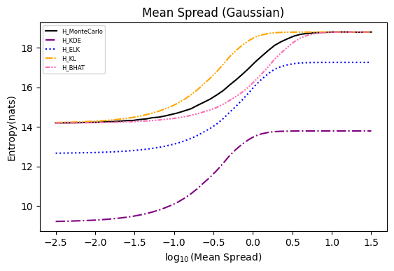
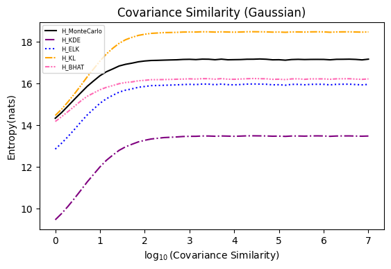
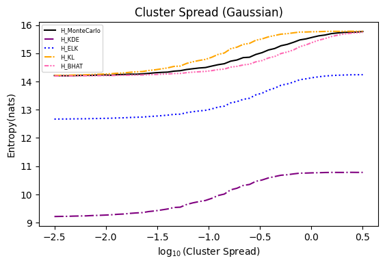
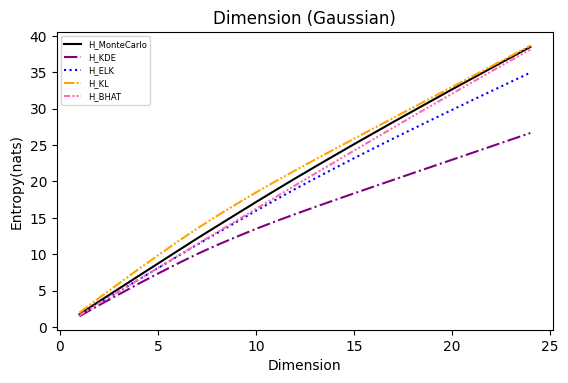
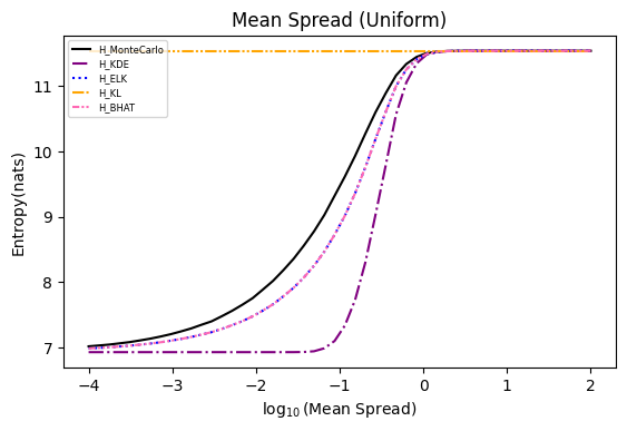
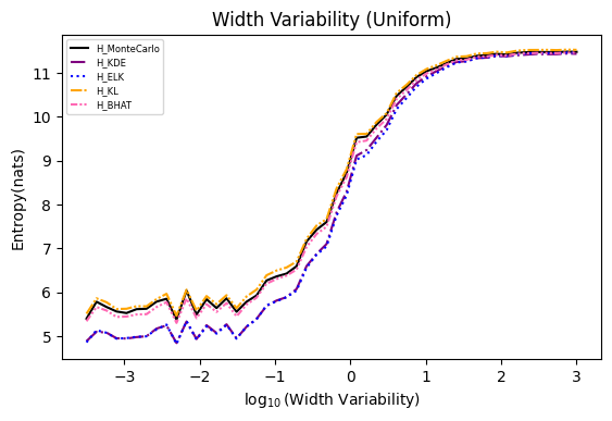
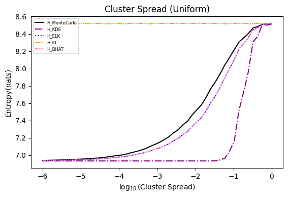
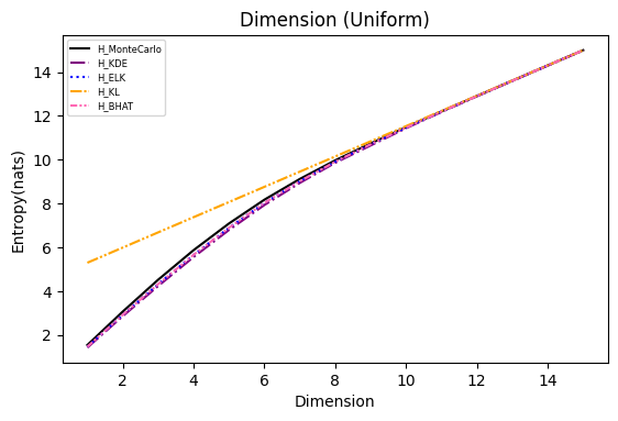
Numerical experiments are performed as described in [3], and following are the results.

NOTE: It is noted in [3] that the x axis of these experiments represents Natural logarithm of the hyperparameter $\ln(\cdot)$, while in the experiments conducted here, the result plot aligns with those presented in the paper using $\log_{10}(\cdot)$.

Also, please refer to [8] for the official implementation in Golang.

References

[1] Joe, H. (1989). Estimation of entropy and other functionals of a multivariate density. Annals of the Institute of Statistical Mathematics, 41, 683-697.

[2] Jebara, T., Kondor, R., & Howard, A. (2004). Probability product kernels. The Journal of Machine Learning Research, 5, 819-844.

[3] Kolchinsky, A., & Tracey, B. D. (2017). Estimating mixture entropy with pairwise distances. Entropy, 19(7), 361.

[4] https://en.wikipedia.org/wiki/Differential_entropy

[5] https://en.wikipedia.org/wiki/Kernel_density_estimation

[6] Zhouyin, Z., & Liu, D. (2021). Understanding neural networks with logarithm determinant entropy estimator. arXiv preprint arXiv:2105.03705.

[7] Cover, T. M. (1999). Elements of information theory. John Wiley & Sons.

[8] https://github.com/btracey/mixent/tree/master

[9] https://en.wikipedia.org/wiki/Bhattacharyya_distance

[10] https://en.wikipedia.org/wiki/Kullback%E2%80%93Leibler_divergence