| aspectratio | author | colorlinks | fonttheme | innertheme | institute | lang | monofont | outertheme | sansfont | theme | title | |
|---|---|---|---|---|---|---|---|---|---|---|---|---|
169 |
Jeremy Theler |
true |
jeremy@seamplex.com |
professionalfonts |
rectangles |
Mid-term evaluation, PhD in Nuclear Engineering
Instituto Balseiro, San Carlos de Bariloche, Argentina
|
en-US |
DejaVuSansMono |
number |
Carlito |
default |
A free and open source computational tool
for solving differential equations in the cloud
|
How do we write papers/reports/documents?
| Feature | ||||
|---|---|---|---|---|
| Aesthetics | ||||
| Convertibility | ||||
| Traceability | ||||
| Mobile-friendliness | ||||
| Collaborative | ||||
| Licensing/openness | ||||
| Non-nerd friendliness |
How do we do scientific/engineering computations?
| Feature | ||||
|---|---|---|---|---|
| Flexibility | ||||
| Scalability | ||||
| Traceability | ||||
| Cloud-friendliness | ||||
| Collaborative | ||||
| Licensing/openness | ||||
| Non-nerd friendliness |
Software Requirement Specifications
After a successful project with a foreign company I decided to structure the PhD based on a fictitious & imaginary “Request for Quotation” for a computational tool:
- Introduction
- 1.1. Objective
- 1.2. Scope
- Architecture
- 2.1. Deployment
- 2.2. Execution
- 2.3. Efficiency
- 2.4. Scalability
- 2.5. Flexibility
- 2.6. Extensibility
- 2.7. Interoperability
- Interfaces
- 3.1. Problem input
- 3.2. Results output
- Quality assurance
- 4.1. Reproducibility and traceability
- 4.2. Automated testing
- 4.3. Bug reporting and tracking
- 4.4. Verification
- 4.5. Validation
- 4.6. Documentation
FeenoX Software Design Specifications
- A fictitious & imaginary tender applying to the SRS addressing each section.
1. Introduction
- Application to industrial problems
- Open source (to allow third-party V&V)
- First version should handle some problems
- Extensible to other problems & formulations
- Free (as in freedom to hire somebody to modify/extend it)
1.1. Objective
- Solve DAEs and/or PDEs
- Heat conduction
- Elasticity
- Electromagnetism
- Fluid mechanics
- …
- State-of-the-art cloud friendly
. . .
FeenoX
- Free as “software libre”
- GPLv3+
- Only FOSS dependencies
- Main target is
linux-x86_64 - Development environment is Debian
- Initial version supports
- Dynamical systems (DAE)
- Laplace/Poisson/Helmholtz (FEM)
- Heat (FEM)
- Elasticity (FEM)
- Modal (FEM)
- Neutron transport and diffusion (FEM/FVM)
- Templates for more formulations
- Electromagnetism
- Chemical diffusion/reaction
- Fluid mechanics?
1.2. Scope
- The problem should be defined programatically
- One or more input files (JSON, YAML, ad-hoc format), and/or
- An API for high-level language (Python, Julia, etc.)
- There is no need to include a GUI
- The tool should allow a GUI to be used
- Desktop
- Web
- Mobile
- The tool should allow a GUI to be used
- The mesh can be an input
- As long as its creation meets the SRS
- Include documentation about how a…
- Pre-processor should create inputs
- Post-processor should read outputs
. . .
FeenoX
- No GUI, console binary executable
- “Transfer-function”-like between I/O
-
No need to recompile the binary

-
- English-like syntactic-sugared input files
- Nouns are definitions
- Verbs are instructions
- Python & Julia API:
- But already taken into account in the design & implementation
- Separate mesher
- Gmsh (GPLv2, meets SRS)
- Anything that writes
.msh
- Possibility to use GUI
- CAEplex https://www.caeplex.com
Transfer-function & English-like input: Lorenz’ system
Solve $$ \begin{cases} \dot{x} = \sigma \cdot (y - x) \\ \dot{y} = x \cdot (r - z) - y \\ \dot{z} = x y - b z \end{cases} $$
for 0 < t < 40 with initial conditions
and σ = 10, r = 28 and b = 8/3.
. . .
PHASE_SPACE x y z
end_time = 40         # dimensionless time

sigma = 10            # parameters
r = 28
b = 8/3

x_0 = -11             # initial conditions
y_0 = -16
z_0 = 22.5

# Lorenz's equations as written in 1963
x_dot = sigma*(y - x)
y_dot = x*(r - z) - y
z_dot = x*y - b*z

PRINT %e t x y z      # four-column plain-ASCII output
$ feenox lorenz.fee
0.000000e+00    -1.100000e+01   -1.600000e+01   2.250000e+01
2.384186e-07    -1.100001e+01   -1.600001e+01   2.250003e+01
4.768372e-07    -1.100002e+01   -1.600002e+01   2.250006e+01
[...]
3.997567e+01    4.442995e+00    3.764391e+00    2.347301e+01
3.998290e+01    4.399950e+00    3.886609e+00    2.314602e+01
3.999012e+01    4.368713e+00    4.016860e+00    2.282821e+01
$
Lorenz’ system

Web interface: CAEplex, finite elements in the cloud

https://www.seamplex.com/feenox/videos/caeplex-ipad.mp4
2. Architecture
- Should run on mainstream cloud servers
- GNU/Linux
- Multi-core Intel-compatible CPUs
- Several levels of memory cache
- A few Gb of RAM
- Several Gb of SSD
- Either
- Bare metal
- Virtualized
- Containerized
- Standard compilers, libraries and dependencies
- Available in common GNU/Linux repositories
- Preferable 100% open source
- Adhere to well-established standards
. . .
FeenoX
-
Third-system effect (after v1 & v2)
-
philosophy: “do one thing well”
- : no GUI
- : Gnuplot, Gmsh, …
- …more rules to come!
-
Third-party math libraries
-
GNU GSL, PETSc, SLEPc, SUNDIALS
-
-
Dependencies available in APT
apt-get install git gcc make automake autoconf apt-get install libgsl-dev apt-get install lib-sundials-dev petsc-dev slepc-dev -
Sources on github.com/seamplex/feenox
git clone https://github.com/seamplex/feenox -
Autotools & friends for compilation
./autogen.sh && ./configure && make
2. Architecture
- Small coarse problems should be run in single hosts to check inputs
- Local desktop/laptops (not needed but suggested)
- Windows and MacOS (not needed but suggested)
- Small cloud instances
- Large actual problems should be split into several hosts
- HPC clusters
- Scalable cloud instances
- Mobile devices (not needed but suggested)
- As control/monitoring devices
. . .
FeenoX
-
Tested on
- Raspberry Pi
- Laptop (GNU/Linux & Windows 10)
- Macbook
- Desktop PC
- Bare-metal servers
- Vagrant/Virtualbox
- Docker/Kubernetes
- AWS/DigitalOcean/Contabo
-
Parallelization:
- Gmsh partitioning with METIS
- PETSc/SLEPc with MPI
-
Web: https://www.caeplex.com (v2)


-
Mobile:
How to solve a maze without AI 1/3


-
Create a maze
-
Download it in PNG
-
Perform some conversions
- PNG → PNM → SVG → DXF → GEO
$ wget http://www.mazegenerator.net/static/orthogonal_maze_with_20_by_20_cells.png
$ convert orthogonal_maze_with_20_by_20_cells.png \
  -negate maze.png
$ potrace maze.pnm --alphamax 0  --opttolerance 0 \
  -b svg -o maze.svg
$ ./svg2dxf maze.svg maze.dxf
$ ./dxf2geo maze.dxf 0.1
How to solve a maze without AI 2/3
-
Open it with Gmsh
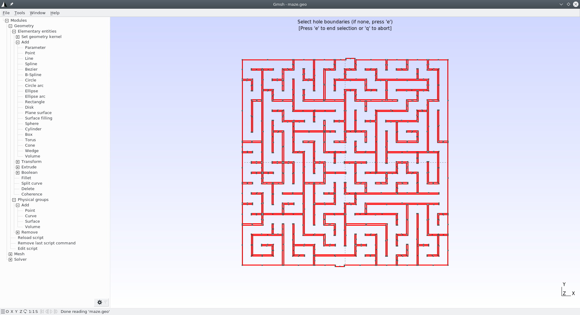
- Add a surface
- Set physical curves for “start” and “end”
-
Mesh it
gmsh -2 maze.geo

How to solve a maze without AI 3/3
-
Solve ∇2ϕ = 0 with BCs $$ \begin{cases} \phi=0 & \text{at “start”} \\ \phi=1 & \text{at “end”} \\ \nabla \phi \cdot \hat{\mathbf{n}} = 0 & \text{everywhere else} \\ \end{cases} $$
PROBLEM laplace 2D  # pretty self-descriptive, isn't it?
READ_MESH maze.msh

# boundary conditions (default is homogeneous Neumann)
BC start  phi=0
BC end    phi=1

SOLVE_PROBLEM

# write the norm of gradient as a scalar field
# and the gradient as a 2d vector into a .msh file
WRITE_MESH maze-solved.msh \
    sqrt(dphidx(x,y)^2+dphidy(x,y)^2) \
    VECTOR dphidx dphidy 0
$ feenox maze.fee $ -
Go to start and follow the gradient ∇ϕ!
The life of an influencer…


2.1. Deployment
- Automatically compile from source
- Particular optimization flags
- Availability of pre-compiled binaries
- Common architectures and options
- Both of them have to be available online
2.2. Execution
- Remote execution, either
- By a direct user action
- From a higher-level workflow
- Outer loops have to be supported
- scripted
- parametric
- optimization
- Ways to read data from the outer loop
- Ways to write scalar figures of merit
. . .
FeenoX
-
Compile optimized dependencies
$ cd $PETSC_DIR $ export PETSC_ARCH=linux-fast $ ./configure --with-debug=0 COPTFLAGS="-Ofast" $ make -j8 -
Configure FeenoX with particular flags
$ git clone https://github.com/seamplex/feenox $ cd feenox $ ./autogen.sh $ export PETSC_ARCH=linux-fast $ ./configure MPICH_CC=clang CFLAGS=-Ofast $ make -j8 # make install -
Or use pre-compiled binaries
wget http://gmsh.info/bin/Linux/gmsh-Linux64.tgz wget https://seamplex.com/feenox/dist/linux/feenox-linux-amd64.tar.gz -
Everything is Docker-friendly
-
Execution examples follow →
Direct execution: three ways of getting the first 20 Fibonacci numbers
# the Fibonacci sequence using the closed-form formula as a function
phi = (1+sqrt(5))/2
f(n) = (phi^n - (1-phi)^n)/sqrt(5)
PRINT_FUNCTION f MIN 1 MAX 20 STEP 1
. . .
# the fibonacci sequence as a vector
VECTOR f SIZE 20

f[i]<1:2> = 1
f[i]<3:vecsize(f)> = f[i-2] + f[i-1]

PRINT_VECTOR i f
. . .
# the fibonacci sequence as an iterative problem

static_steps = 20
#static_iterations = 1476  # limit of doubles

IF step_static=1|step_static=2
 f_n = 1
 f_nminus1 = 1
 f_nminus2 = 1
ELSE
 f_n = f_nminus1 + f_nminus2
 f_nminus2 = f_nminus1
 f_nminus1 = f_n
ENDIF

PRINT step_static f_n
. . .
$ feenox fibo_formula.fee | tee one
1   1
2   1
3   2
4   3
5   5
6   8
7   13
8   21
9   34
10  55
11  89
12  144
13  233
14  377
15  610
16  987
17  1597
18  2584
19  4181
20  6765
$ feenox fibo_vector.fee > two
$ feenox fibo_iterative.fee > three
$ diff one two
$ diff two three
$
Parametric execution: shear locking in cantilevered beam
#!/bin/bash

rm -f *.dat
for element in tet4 tet10 hex8 hex20 hex27; do
 for c in $(seq 1 10); do

  # create mesh if not alreay cached
  mesh=cantilever-${element}-${c}
  if [ ! -e ${mesh}.msh ]; then
    scale=$(echo "PRINT 1/${c}" | feenox -)
    gmsh -3 -v 0 cantilever-${element}.geo -clscale ${scale} -o ${mesh}.msh
  fi

  # call FeenoX
  feenox cantilever.fee ${element} ${c} | tee -a cantilever-${element}.dat

 done
done
PROBLEM elastic 3D
READ_MESH cantilever-$1-$2.msh # in meters
E = 2.1e11 # Young modulus in Pascals
nu = 0.3 # Poisson's ratio
BC left fixed
BC right tz=-1e5 # traction in Pascals, negative z
SOLVE_PROBLEM
# z-displacement (components are u,v,w) at the tip vs. number of nodes
PRINT nodes w(500,0,0) "\# $1 $2"


-
- Only one material, no need to link volumes with materials
E = 2.1e11 # Young modulus in Pa
Parametric execution: shear locking in cantilevered beam
Optimization loop: finding the right length of a tuning fork

ℓ1 to have 440 Hz?
. . .
import math
import gmsh
import subprocess  # to call FeenoX and read back

def create_mesh(r, w, l1, l2, n):
  gmsh.initialize()
  ...
  gmsh.finalize()
  return len(nodes)

def main():
  target = 440    # target frequency
  eps = 1e-2      # tolerance
  r = 4.2e-3      # geometric parameters
  w = 3e-3
  l1 = 30e-3
  l2 = 60e-3

  for n in range(1,7):   # mesh refinement level
    l1 = 60e-3              # restart l1 & error
    error = 60
    while abs(error) > eps:   # loop
      l1 = l1 - 1e-4*error
      # mesh with Gmsh Python API
      nodes = create_mesh(r, w, l1, l2, n)
      # call FeenoX and read scalar back
      # TODO: FeenoX Python API (like Gmsh)
      result = subprocess.run(['feenox', 'fork.fee'], stdout=subprocess.PIPE)
      freq = float(result.stdout.decode('utf-8'))
      error = target - freq

    print(nodes, l1, freq)
PROBLEM modal 3D MODES 1 # only one mode needed
READ_MESH fork.msh # in [m]
E = 2.07e11 # in [Pa]
nu = 0.33
rho = 7829 # in [kg/m^2]
# no BCs! It is a free-free vibration problem
SOLVE_PROBLEM
# write back the fundamental frequency to stdout
PRINT f(1)
. . .
$ python fork.py > fork.dat
$
2.3. Efficiency
- Similar to to other tools in terms of
- CPU/GPU
- RAM
- Storage
2.4. Scalability
- Small problems to check correctness
- Large problems in parallel
- Reasonable weak & strong scalability
2.5. Flexibility
- Engineering problems with
- Multiple materials
- Space-dependent properties
- Space & time-dependent BCs
- Handle point-wise data
- Properties
- Time-dependent scalars
. . .
FeenoX
-
First make it work, then optimize
- Premature optimization is the root of all evil
- Optimization:
- Parallelization:
- Comparison:
- Linear solvers
- Direct solver MUMPS
- Robust but not scalable
- GAMG-preconditioned KSP
- Near-nullspace improves convergence
- Direct solver MUMPS
- Non-linear & transient solvers
- Scalable as PETSc
- Written in ANSI C99 (no C++ nor Fortran)
-
Autotools & friends, POSIX
-
Tested with
gcc,clangandicc -
Rust & Go, can’t tell (yet)
-
- Flexibility follows →
Flexibility I: one-dimensional thermal slab
Solve heat conduction on the slab x ∈ [0:1] with boundary conditions
and uniform conductivity. Compute
. . .
- English self-evident ASCII input
- Syntactic sugar
- Simple problems, simple inputs
- Robust (
heatorthermal)
- Mesh separated from problem
- Git-friendly
.geo&.fee
- Git-friendly
- Output is 100% user-defined
-
No
PRINTno output
-
- There is no node at x = 1/2 = 0.5!
Point(1) = {0, 0, 0};          // geometry:
Point(2) = {1, 0, 0};          // two points
Line(1) = {1, 2};              // and a line connecting them!

Physical Point("left") = {1};  // groups for BCs and materials
Physical Point("right") = {2};
Physical Line("bulk") = {1};   // needed due to how Gmsh works

Mesh.MeshSizeMax = 1/3;        // mesh size, three line elements
Mesh.MeshSizeMin = Mesh.MeshSizeMax;
PROBLEM thermal 1D # tell FeenoX what we want to solve
READ_MESH slab.msh # read mesh in Gmsh's v4.1 format
k = 1 # set uniform conductivity
BC left T=0 # set fixed temperatures as BCs
BC right T=1 # "left" and "right" are defined in the mesh
SOLVE_PROBLEM # we are ready to solve the problem
PRINT T(1/2) # ask for the temperature at x=1/2
$ gmsh -1 slab.geo
[...]
Info    : 4 nodes 5 elements
Info    : Writing 'slab.msh'...
[...]
$ feenox thermal-1d-dirichlet-uniform-k.fee
0.5
$
Flexibility II: one-dimensional thermal slabs
PROBLEM heat 1D
READ_MESH slab.msh

BC left  T=0
BC right T=1

INCLUDE $1.fee   # read k and solution from $1

SOLVE_PROBLEM

PRINT_FUNCTION T T_analytical MIN 0 MAX 1 NSTEPS 100
k = 1            # uniform.fee
T_analytical(x) = x
k(x) = 1+x       # space.fee
T_analytical(x) = log(1+x)/log(2)
a = 2            # temperature.fee
k(x) = 1+a*T(x)
T_analytical(x) = (1/a)*(sqrt(1+(2+a)*a*x)-1)
. . .
- Everything is an expression
- Similar problems need similar inputs
- : k(x) = 1 + x
Flexibility III: two squares in thermal contact

PROBLEM thermal 2d
READ_MESH two-squares.msh

FUNCTION cond(x,y) INTERPOLATION shepard DATA {
    1   0    1.0
    1   1    1.5
    2   0    1.3
    2   1    1.8
    1.5 0.5  1.7 }

#        name   conductivity  power density
MATERIAL yellow k=0.5+T(x,y)  q=0
MATERIAL cyan   k=cond(x,y)   q=1-0.2*T(x,y)

BC left   T=y              # temperature
BC bottom T=1-cos(pi/2*x)
BC right  q=2-y            # heat flux
BC top    q=1

SOLVE_PROBLEM

WRITE_MESH two-squares.vtk  T CELLS k
. . .


- Volumes ⇔ materials now needed
- FeenoX detects the problem is non-linear
- : roughish output
Flexibility IV: thermal transient with time-dependent BCs

. . .
# NAFEMS-T3 benchmark: 1d transient heat conduction
PROBLEM heat DIMENSIONS 1
READ_MESH slab-0.1m.msh

T_0(x) = 0         # initial condition

BC left  T=0       # prescribed temperatures
BC right T=100*sin(pi*t/40)

k = 35.0           # conductivity [W/(m K)]
cp = 440.5         # heat capacity [J/(kg K)]
rho = 7200         # density [kg/m^3]

end_time = 32      # trasient up to 32 seconds

SOLVE_PROBLEM

PRINT %.3f t dt %.2f T(0.1) T(0.08)

IF done
 PRINT "\# result = " T(0.08) "ºC"
ENDIF
$ feenox nafems-t3.fee
0.000   0.062   0.00    0.00
0.002   0.002   0.01    0.00
[...]
30.871  0.565   65.71   36.04
31.435  0.565   62.31   36.33
32.000  1.050   58.78   36.56
# result =      36.5636 ºC
$
Flexibility V: 3D thermal transient with k(x)

https://www.seamplex.com/feenox/videos/temp-valve-smooth.mp4
Flexibility VI: point kinetics with point-wise reactivity
| t [s] | ρ(t) [pcm] |
|---|---|
| 0 | 0 |
| 5 | 0 |
| 10 | 10 |
| 30 | 10 |
| 35 | 0 |
| 100 | 0 |
for 0 < t < 100 starting from steady-steate conditions at full power.
. . .
INCLUDE parameters.fee    # kinetic parameters

# our phase space is flux, precursors and reactivity
PHASE_SPACE phi c rho

end_time = 100
# we need a tighter error to handle small reactivities
rel_error = 1e-7

# steady-state initial conditions
rho_0 = 0   # no reactivity
phi_0 = 1   # full power
c_0[i] = phi_0 * beta[i]/(Lambda*lambda[i])

FUNCTION react(t) DATA {   0    0   # in pcm
                           5    0
                           10  10
                           30  10
                           35   0
                           100  0   }

# reactor point kinetics equations
rho = 1e-5*react(t)   # convert pcm to absolute
phi_dot = (rho-Beta)/Lambda * phi + vecdot(lambda, c)
c_dot[i] = beta[i]/Lambda * phi - lambda[i]*c[i]

PRINT t phi rho
$ feenox reactivity-from-table.fee > flux.dat
$
Flexibility VI: inverse kinetics
INCLUDE parameters.fee
FUNCTION flux(t) FILE_PATH $1  # read flux from file

# define a flux function that allow for negative times
t_min = vec_flux_t[1]
t_max = vec_flux_t[vecsize(vec_flux)]
phi(t) := if(t<t_min, flux(t_min), flux(t))

VAR t'   # dummy integration variable
# compute the reactivity with the integral formula
rho(t) := Lambda * derivative(log(phi(t')),t',t) + Beta * ( 1 - 1/phi(t) * integral(phi(t-t') * sum((lambda[i]*beta[i]/Beta)*exp(-lambda[i]*t'), i, 1, nprec), t', 0, 1e4) )

PRINT_FUNCTION rho MIN t_min MAX t_max STEP (t_max-t_min)/1000
. . .
INCLUDE parameters.fee
PHASE_SPACE phi c rho

end_time = 100
rel_error = 1e-7

rho_0 = 0
phi_0 = 1
c_0[i] = phi_0 * beta(i)/(Lambda*lambda(i))

FUNCTION flux(t) FILE $1
phi = flux(t) # force the variable phi to the data
phi_dot = (rho-Beta)/Lambda * phi + vecdot(lambda, c)
c_dot[i] = beta[i]/Lambda * phi - lambda[i]*c[i]

PRINT t phi rho
. . .
$ feenox inverse-dae.fee flux.dat > inverse-dae.dat
$ feenox inverse-integral.fee flux.dat > inverse-integral.dat
2.6. Extensibility
- Possibility to add more features
- More PDEs
- New material models (i.e. stress-strain)
- Other element types
- Clear licensing scheme for extensions
2.7. Interoperability
- Ability to exchange data with other tools following this SRS
- Pre and post processors
- Optimization tools
- Coupled multi-physics calculations
. . .
FeenoX
- Think for the future!
- GPLv3**+**: the ‘+’ is for the future
- Nice-to-haves:
- Lagrangian elements, DG, h-p AMR, …
- Other problems & formulations:
- Each PDE has an independent directory
- “Virtual methods” as function pointers
- Use Laplace as a template (elliptic)
- Coupled calculations:
- Wide experience from CNA2 (v2)
- Plain (RAM-disk) files
- Shared memory & semaphores
- MPI
- Interoperability
- Gnuplot, matplotlib, etc.
- Gmsh (+ Meshio), Paraview
- CAEplex
- PrePoMax, FreeCAD, …:
Laplace equation with both Gmsh & Paraview as post-processors
Solve ∇2ϕ = 0 over [−1:+1] × [−1:+1] with
PROBLEM laplace 2d
READ_MESH square-centered.msh # [-1:+1]x[-1:+1]

# boundary conditions
BC left    phi=+y
BC right   phi=-y
BC bottom  dphidn=sin(pi/2*x)
BC top     dphidn=0

SOLVE_PROBLEM

# same output in .msh and in .vtk formats
WRITE_MESH laplace-square.msh phi VECTOR dphidx dphidy 0
WRITE_MESH laplace-square.vtk phi VECTOR dphidx dphidy 0
. . .


3. Interfaces
- Fully human-less execution
- Input files (1 or more)
- Output files (0 or more)
- Ability to remotely report status
- Progress
- Errors
3.1. Input
- Problem fully defined in input files
- Ad-hoc syntax
- API for high-level languages
- Other files (data, meshes, scripts)
- Preferably ASCII (for DCVS)
- Avoid mixing problem and mesh data
- GUI not mandatory but possible
- Ok to have basic usage through GUI
- Advanced features through API
. . .
FeenoX
-
Already deployed industrial human-less production workflow (based on v2)
-
There are ASCII progress bars
- Build matrix
- Solve equations
- Gradient recovery
-
Heartbeat:
-
English self-evident ASCII input
-
Syntactically-sugared
- Nouns are definitions
- Verbs are instructions
-
Simple problems, simple inputs
-
Similar problems, similar inputs
-
Everything is an expression!
-
:
$f(x)=\frac{1}{2} \cdot x^2$ f(x) = 1/2 * x^2 -
Expansion of command line arguments
-
CAEplex progress status on the cloud

https://www.seamplex.com/feenox/videos/caeplex-progress.mp4
NAFEMS LE10: English-like problem definition & user-defined output

. . .
# NAFEMS Benchmark LE-10: thick plate pressure
PROBLEM mechanical DIMENSIONS 3
READ_MESH nafems-le10.msh   # mesh in millimeters

# LOADING: uniform normal pressure on the upper surface
BC upper    p=1      # 1 Mpa

# BOUNDARY CONDITIONS:
BC DCD'C'   v=0      # Face DCD'C' zero y-displacement
BC ABA'B'   u=0      # Face ABA'B' zero x-displacement
BC BCB'C'   u=0 v=0  # Face BCB'C' x and y displ. fixed
BC midplane w=0      #  z displacements fixed along mid-plane

# MATERIAL PROPERTIES: isotropic single-material properties
E = 210e3   # Young modulus in MPa
nu = 0.3    # Poisson's ratio

SOLVE_PROBLEM   # solve!

# print the direct stress y at D (and nothing more)
PRINT "sigma_y @ D = " sigmay(2000,0,300) "MPa"
$ gmsh -3 nafems-le10.geo
[...]
Info    : Done meshing order 2 (Wall 0.433083s, CPU 0.414008s)
Info    : 205441 nodes 59892 elements
Info    : Writing 'nafems-le10.msh'...
$ feenox nafems-le10.fee
sigma_y @ D =  -5.38361 MPa
$
NAFEMS LE11: everything is an expression (especially temperature)

. . .
PROBLEM mechanical 3D
READ_MESH nafems-le11.msh

# linear temperature gradient in the radial and axial direction
T(x,y,z) := sqrt(x^2 + y^2) + z  # UTEMP for this????

BC xz     v=0       # displacement vector is [u,v,w]
BC yz     u=0       # u = displacement in x
BC xy     w=0       # v = displacement in y
BC HIH'I' w=0       # w = displacement in z

E = 210e3*1e6       # mesh is in meters, so E=210e3 MPa -> Pa
nu = 0.3            # dimensionless
alpha = 2.3e-4      # in 1/ºC as in the problem
SOLVE_PROBLEM

# for post-processing in Paraview
WRITE_MESH nafems-le11.vtk VECTOR u v w   T sigmax sigmay sigmaz

PRINT "sigma_z(A) = " sigmaz(0,1,0)/1e6 "MPa" SEP " "
$ gmsh -3 -clscale 0.5 nafems-le11.geo
[...]
Info    : 8326 nodes 1849 elements
Info    : Writing 'nafems-le11.msh'...
$ feenox nafems-le11.fee
sigma_z(A) =  -105.043 MPa
$
3.2. Output
- Clean output expected
- Do not clutter the output with
- ASCII art
- Notices
- Explanations
- Page separators
- Output should interpreted by both
- A human
- A computer
- Open standards and well-documented formats should be preferred
. . .
FeenoX
- : output is completely defined by the user
- : no
PRINTno output - ASCII columns
PRINT&PRINT_FUNCTION- Gnuplot & compatible
- Markdown/LaTeX tables
- Post-processing formats
.msh.vtk.vtu:.hdf5:.frd: ?
- Dumping of vectors & matrices
- ASCII
- PETSc binary
- Octave (sparse)
100% user-defined output: cycle loads
For the model below, draw the sequence of loading and unloading for different levels of strains. All bars have the same geometry and elastic properties but different yield stresses.

for i in 1 2 3 4; do
  feenox 3bars.fee ${i}
  pyxplot 3bars.ppl
  mv 3bars-sigma-vs-eps.pdf 3bars-sigma-vs-eps-${i}.pdf
done
DEFAULT_ARGUMENT_VALUE 1 5
E = 1 # non-dimensional Young modulus
yield1 = 3.5 # non-dimensional yield stresses
yield2 = 2.5
yield3 = 1.5
eps_max = $1 # max strain from command line
end_time = 2*eps_max
PHASE_SPACE eps sigma1 sigma2 sigma3 P
eps_0 = 0 # initial conditions
sigma1_0 = 0
sigma2_0 = 0
sigma3_0 = 0
P_0 = 0
# DAEs
eps = eps_max * sin(3*pi*t/end_time)
sigma1_dot = E * eps_dot * if((eps_dot < 0 | sigma1 < yield1) & (eps_dot > 0 | sigma1 > (-yield1)))
sigma2_dot = E * eps_dot * if((eps_dot < 0 | sigma2 < yield2) & (eps_dot > 0 | sigma2 > (-yield2)))
sigma3_dot = E * eps_dot * if((eps_dot < 0 | sigma3 < yield3) & (eps_dot > 0 | sigma3 > (-yield3)))
P = sigma1 + sigma2 + sigma3
PRINT FILE 3bars.dat t eps P sigma1 sigma2 sigma3
100% user-defined output: cycle loads
Markdown table: natural oscillation frequencies of a wire
Experimental Physics 101 (2004)

# compare the frequencies
PRINT "  \$n\$ |   FEM  | Euler | Relative difference [%]"
PRINT ":----:+:------:+:-----:+:-----------------------:"
PRINT_VECTOR i         f(2*i-1) f_euler   100*(f_euler(i)-f(2*i-1))/f_euler(i)
PRINT
PRINT ": $2 wire over $1 mesh, frequencies in Hz"
$ feenox wire.fee copper hex > copper-hex.md
$
| n | FEM | Euler | Relative difference [%] |
|---|---|---|---|
| 1 | 45.8374 | 45.8448 | 0.0161707 |
| 2 | 287.126 | 287.302 | 0.0611787 |
| 3 | 803.369 | 804.454 | 0.134888 |
| 4 | 1572.59 | 1576.41 | 0.242324 |
| 5 | 2595.99 | 2605.92 | 0.381107 |
copper wire over hex mesh, frequencies in Hz
Professional tables: environmentally-assisted fatigue


-
Computation of NUREG-EPRI sample problem for Environmentally-assisted fatigue in NPP piping
-
Top is a table from a publication by a multi-billion dollar agency
-
Bottom is a PDF from FeenoX output piped through
- AWK
Data for videos I: four double pendulums (v2)

https://www.seamplex.com/feenox/videos/pendulums.webm
Data for videos II: boiling channel with sinusoidal power profile (v2)

https://www.seamplex.com/feenox/videos/sine.webm
Data for videos III: modal analysis for seismic analysis of piping (v2)

https://www.seamplex.com/feenox/videos/mode5.mp4 https://www.seamplex.com/feenox/videos/mode6.mp4 https://www.seamplex.com/feenox/videos/mode7.mp4
Complex figures: 2D IAEA PWR Benchmark (v2)
Complex figures: 2D IAEA PWR Benchmark (v2)
Core-level neutronics over unstructured grids: the S2 Stanford Bunny (v2)

- One-group neutron transport
- The Stanford Bunny as the geometry
- S2 method in 3D (8 angular directions)
- Finite elements for spatial discretization


4. Quality Assurance
- Generic good software QA practices
- Distributed version control system
- Automated testing suites
- User-reported bug tracking support
- Signed releases
- etc.
4.1. Reproducibility and traceability
- Both the source and the documentation should be tracked with a DVCS
- Repository should be accessible online
- Might need credentials even for RO
- Version reporting
- Executables must allow
--version - Libraries must provide an API call
- Executables must allow
- The files needed to solve a problem should be simple & traceable by a DVCS
. . .
FeenoX
- Hosted on Github (
git)- Previously on Bitbucket (
hg) - Previously on Launchpad (
bzr) - Previously on-premise (
svn)
- Previously on Bitbucket (
- https://github.com/seamplex/feenox
- https://seamplex.com/feenox
- Mailing list (Google group)
- Build a community!
- Code of conduct
$ feenox
FeenoX v0.1.12-gb9a534f-dirty
a free no-fee no-X uniX-like finite-element(ish) computational engineering tool

usage: feenox [options] inputfile [replacement arguments]
[...]
$
-
-v/--version: copyright notice -
-V/--versions: linked libraries -
: inputs from M4
4.2. Automated testing
- A mean to test the code is mandatory
- After each change
- Check for regressions
- Problems with already-computed solutions
- Different from verification
- The compiler should not issue warnings
- Dynamic memory allocation checks are recommended
- Good practices are suggested
- Unit testing
- Continuous integration
- Test coverage analysis
4.3. Bug reporting and tracking
- Users should be able to report bugs
- A task should be created for each report
- Address and document
. . .
FeenoX
-
Standard test suite
$ make check Making check in src [...] PASS: tests/trig.sh PASS: tests/vector.sh ============================================= Testsuite summary for feenox v0.1.12-gb9a534f ============================================= # TOTAL: 26 # PASS: 25 # SKIP: 0 # XFAIL: 1 # FAIL: 0 # XPASS: 0 # ERROR: 0 ============================================= $ -
Periodic
valgrindruns -
Integration tests:
-
CI & test coverage:
-
Github issue tracker
-
Branching & merging procedures:
4.4 Verification
- Code must be always verified
- Check it solves right the equations
- MES (mandatory)
- MMS (recommended)
- One test case has to be added to the automated testing
- Third-party verification should be allowed
- Per-problem documentation
4.5. Validation
- Code should be validated as required
- Check it solves the right equations
- Against experiments
- Against other codes
- Third-party validation should be allowed
- Per-application/industry documentation
- Procedures following standards
. . .
FeenoX
-
There is a V&V report for the industrial human-less workflow project
- Medical devices
- Based on ASME V&V 40
-
There is a lot to do!
-
MES
- Set of well-known benchmarks
- NAFEMS, IAEA, etc.
-
MMS
- Everything is an expression
- Parametric runs
MESH_INTEGRATEallows to compute L2 norms directly in the.fee
-
TL;DR:
Experimental Validation

https://fusor.net/board/viewtopic.php?f=13&t=14087 ← because it is FOSS!
4.6. Documentation
- Documentation should be complete
- User manual
- Tutorial
- Reference
- Developer guide
- User manual
- Quick reference cards, video tutorials, etc. not mandatory but recommended
- Non-trivial mathematics and methods
- Explained
- Documented
- Should be available as hard copies and mobile-friendly online
- Clear licensing scheme for the documentation
- People extending the functionality ought to be able to document their work
FeenoX
-
FeenoX is not compact!
- Even I have to check the reference
-
Commented sources:
- Keywords
- Functions
- Functionals
- Variables
- Material properties
- Boundary conditions
- Solutions
-
Shape functions:
-
Gradient recovery:
-
Mathematical models:
-
Code is GPLv3+
-
Documentation is GFDLv1.3+
Conclusions—FeenoX…
- closes a 15-year loop (2006–2021) with a third-system effect
- is to FEA what Markdown is to documentation
- is (so far) the only tool that fulfills 100% a fictitious SRS:
- Free and open source (GPLv3+)
- No recompilation needed
- Cloud and web friendly
- Human-less workflow
- follows the philosophy: “do one thing well”
- is already usable (and used!)
- FeenoX v1.0 coincident with the PhD ()
- Laplace, heat, elasticity, modal, neutron transport & diffusion
- Every current feature is there because there was at least one need from an actual project
- Future versions online ()
- Electromagnetism? CFD? Schrödinger’s equation?
- Python & Julia API
- Coupled & multiphysics computations
- Free and open-source online community
- FeenoX v1.0 coincident with the PhD ()