Panstripe improves the post processing of bacterial pangenome analyses. In particular it aims to replace the dubious but popular pangenome accumulation curve. The package is currently under development so frequent changes are to be expected.
- Installation
- Quick Start
- Citation
- Comparing Pangenomes
- Open vs Closed
- Rate vs Size
- Output
- Alternative models
- Plots
panstripe is currently available on GitHub. It can be installed with
devtools
install.packages("remotes")
remotes::install_github("gtonkinhill/panstripe")
If you would like to also build the vignette with your installation run:
remotes::install_github("gtonkinhill/panstripe", build_vignettes = TRUE)Panstripe takes as input a phylogeny and gene presence/absence matrix in Rtab format as is produced by Panaroo, Roary, PIRATE and other prokaryotic pangenome tools.
library(panstripe)
library(ape)
library(patchwork)
set.seed(1234)

### NOTE: here we load example files from the panstripe package. You should
### replace these variables with the relevant paths to the files you are using.
phylo.file.name <- system.file("extdata", "tree.newick", package = "panstripe")
rtab.file.name <- system.file("extdata", "gene_presence_absence.Rtab", package = "panstripe")
###

# Load files
pa <- read_rtab(rtab.file.name)
tree <- read.tree(phylo.file.name)

# Run panstripe
fit <- panstripe(pa, tree)
fit$summary
#> # A tibble: 6 × 7
#>   term  estimate std.error statistic   p.value `bootstrap CI …` `bootstrap CI …`
#>   <chr>    <dbl>     <dbl>     <dbl>     <dbl>            <dbl>            <dbl>
#> 1 istip   1.49      0.282      5.29   8.03e- 7           0.978             1.99
#> 2 core    2.97      0.247     12.0    9.69e-21           2.54              3.54
#> 3 depth   0.0572    0.0619     0.923  3.58e- 1          -0.0859            0.162
#> 4 isti…  -1.93      0.431     -4.48   2.10e- 5          -2.82             -1.18
#> 5 p       1.25     NA         NA     NA                  1.11              1.36
#> 6 phi     2.58     NA         NA     NA                  1.92              3.28

# Plot results
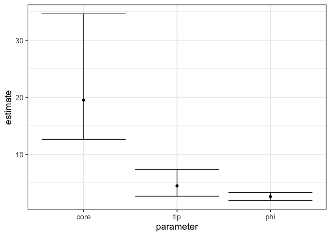
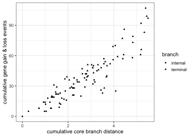
plot_pangenome_params(fit)plot_pangenome_cumulative(fit)A significant p-value for the tip term indicates that there is a
different rate of gene exchange at the tips of the phylogeny compared
with the internal branches. This is usually driven by annotation errors
or highly mobile elements that do not persist long enough to be observed
in multiple genomes.
A significant p-value for the core term indicates that there is a
significant association between the core genome branch length and the
number of gene exchange events.
The depth term is less interesting but indicates when there is a
difference in our ability to detect older gene exchange events.
To cite panstripe please use: Tonkin-Hill, G. et al. Robust analysis of prokaryotic pangenome gene gain and loss rates with Panstripe. bioRxiv (2022) doi:10.1101/2022.04.23.489244
As panstripe uses a GLM framework it is straightforward to compare the
slope terms between datasets. The compare_pangenomes function
considers the interaction term between the data sets and the core,
tip and depth terms.
IMPORTANT: It is important that the phylogenies for the pangenomes being compared are on the same scale. This can be achieved most easily by using time scaled phylogenies. Alternatively, it is possible to build a single phylogeny and partition it into clades or use SNP scaled phylogenies.
Here, we simulate two pangenomes with different gene exhange rates, fit
the model using panstripe and run the compare_pangenomes function.
# Simulate a fast gene gain/loss rate with error
sim_fast <- simulate_pan(rate = 0.001, ngenomes = 200)
sim_slow <- simulate_pan(rate = 5e-04, ngenomes = 200)

# Run panstripe
fit_fast <- panstripe(sim_fast$pa, sim_fast$tree)
fit_slow <- panstripe(sim_slow$pa, sim_slow$tree)

# Compare the fits
result <- compare_pangenomes(fit_fast, fit_slow)
result$summary
#> # A tibble: 4 × 7
#>   term    estimate std.error statistic p.value `bootstrap CI …` `bootstrap CI …`
#>   <chr>      <dbl>     <dbl>     <dbl>   <dbl>            <dbl>            <dbl>
#> 1 depth    -0.0578    0.0268    -2.16  3.14e-2           -0.108          -0.0148
#> 2 istip    -0.0464    0.173     -0.268 7.88e-1           -0.266           0.323
#> 3 core     -0.683     0.165     -4.15  3.74e-5           -0.972          -0.345
#> 4 disper…  NA        NA          0.439 5.08e-1           NA              NA
A significant p-value for the tip term indicates that the two
pangenomes differ in the rates of gene presence and absence assigned to
the tips of the phylogeny. This is usually driven by either differences
in the annotation error rates between data sets or differences in the
gain and loss of highly mobile elements that do not persist long enough
to be observed in multiple genomes.
A significant p-value for the core term indicates that two data sets
have different rates of gene gain and loss.
The depth term is less interesting but indicates when there is a
difference in our ability to detect older gene exchange events between
the two pangenomes.
The dispersion parameter indicates if there is a significant
difference in the dispersion of the two pangenomes. This suggests that
the relationship between the rate of gene exchange and the size of each
event differs in the two pangenomes. Here, the p-value is obtained using
a Likelihood Ratio Test.
## Plot the results

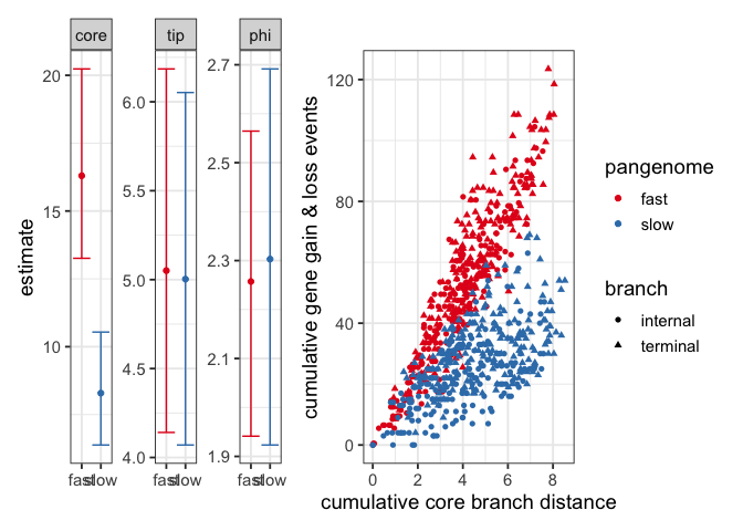
plot_pangenome_params(list(fast = fit_fast, slow = fit_slow), legend = FALSE) + plot_pangenome_cumulative(list(fast = fit_fast,
slow = fit_slow)) + plot_layout(nrow = 1)The definition of what constitutes an open or closed pangenome is somewhat ambiguous. We prefer to consider whether there is evidence for a temporal signal in the pattern of gene gain and loss. This prevents annotation errors leading to misleading results.
After fitting a panstripe model the significance of the temporal
signal can be assessed by considering the coefficient and p-value of the
‘core’ term in the model. The uncertainty of this estimate can also be
investigated by looking at the bootstrap confidence intervals of the
core term.
Let’s simulate a ‘closed’ pangenome
sim_closed <- simulate_pan(rate = 0, ngenomes = 100)
fit_closed <- panstripe(sim_closed$pa, sim_closed$tree)

fit_closed$summary
#> # A tibble: 6 × 7
#>   term  estimate std.error statistic   p.value `bootstrap CI …` `bootstrap CI …`
#>   <chr>    <dbl>     <dbl>     <dbl>     <dbl>            <dbl>            <dbl>
#> 1 istip  1.53e+0   1.43e-1   10.7     3.09e-21            1.13            1.90
#> 2 core  -7.23e+2   3.80e+4   -0.0190  9.85e- 1         -783.           -492.
#> 3 depth -4.52e-2   3.74e-2   -1.21    2.29e- 1           -0.145           0.0549
#> 4 isti…  7.23e+2   3.80e+4    0.0190  9.85e- 1          493.            784.
#> 5 p      1.05e+0  NA         NA      NA                   1.00            1.44
#> 6 phi    3.99e-1  NA         NA      NA                   0.199           0.525
The p-value indicates that there is not a significant association between core branch lengths and gene gain/loss. This is typical of species that undergo very little to no recombination such as M. tuberculosis.
While comparing the core parameter of the model identifies differences
in the association between branch lengths and gene gain and loss it does
not indicate whether this is driven by higher rates of recombination or
simply larger recombination events involving more genes.
The panstripe model allows these two scenarios to be investigated by
allowing the dispersion parameter in the model to be different for each
pangenome.
Here, we simulate two data sets with the same recombination rate but where each recombination event differs in the number of genes involved.
sim_large <- simulate_pan(rate = 0.001, ngenomes = 100, mean_trans_size = 4)
sim_small <- simulate_pan(rate = 0.001, ngenomes = 100, mean_trans_size = 3)

fit_large <- panstripe(sim_large$pa, sim_large$tree)
fit_small <- panstripe(sim_small$pa, sim_small$tree)

# Compare the fits
result <- compare_pangenomes(fit_large, fit_small)
result$summary
#> # A tibble: 4 × 7
#>   term    estimate std.error statistic p.value `bootstrap CI …` `bootstrap CI …`
#>   <chr>      <dbl>     <dbl>     <dbl>   <dbl>            <dbl>            <dbl>
#> 1 depth     0.0858    0.0490     1.75   0.0807          -0.0169            0.201
#> 2 istip    -0.181     0.297     -0.609  0.543           -0.739             0.394
#> 3 core     -0.365     0.226     -1.62   0.106           -0.889             0.121
#> 4 disper… NA NA 6.14 0.0132 NA NAThe panstripe function generates a list with the following attributes
A table indicating a subset of the inferred parameters of the GLM. The p-values and bootstrap confidence intervals can be used to determine whether each term in the model is significantly associated with gene gain and loss.
-
core indicates whether the branch lengths in the phylogeny are associated with gene gain and loss.
-
tip indicates associations with genes observed to occur on the tips of the phylogeny. These are usually driven by a combination of annotation errors and depending upon the temporal sampling density also highly mobile elements that are not observed in multiple genomes.
-
depth indicates whether the rate of gene gain and loss changes significantly with the depth of a branch. Typically, our ability to detect gene exchange events reduces for older ancestral branches.
-
p the inferred index parameter of the underlying Tweedie distribution used in the GLM
-
phi the inferred dispersion parameter of the GLM
The output of fitting the GLM model. This object can be used to predict how many gene gains and losses we would expect to observe given the parameters of a particular branch.
A table with the data used to fit the model. The acc column indicates
the inferred number of gene gain/loss events for a branch; the core
column is the branch length taken from the phylogeny; the istip column
indicates whether the branch occurs at the tip of the phylogeny and the
depth column indicates the distance from the root node to the branch.
A ‘boot’ object, generated by the boot package. Can be used to investigate the uncertainty in the parameter estimates.
The original data provided to the panstripe function.
The default Panstripe model assumes a Compound Poisson (Tweedie) distribution as implemented in the Tweedie R package. In some cases there may be insufficient data or the data may not reliably fit the Tweedie distribution. This is often the case when there is nearly no gene exchange events inferred to have occurred at the internal branches of the phylogeny.
To help account for these issues and to add flexibility to the package it is also possible to fit alternative distributions in place of the Tweedie model. The most common alternative that we suggest is to use a Gaussian distribution. This is usually more robust and is less likely to run into convergence issues in the model fit. In our tests both of these distributions generally give very similar results.
Panstripe can be run using an alternative distribution as
fit_gaussian <- panstripe(pa, tree, family = "gaussian")Panstripe includes a number of useful plotting functions to help with interpretation of the output of panaroo.
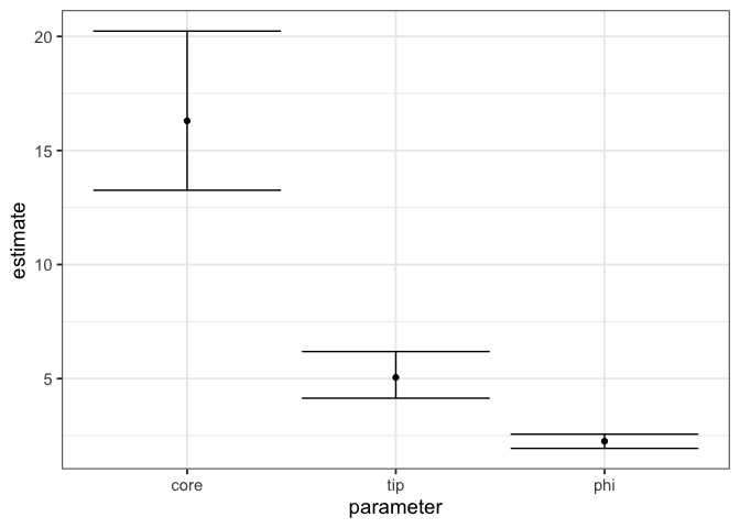
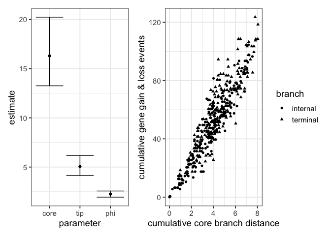
The inferred parameters of the Panstripe model fit can be plotted as
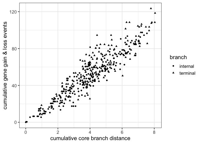
plot_pangenome_params(fit_fast)We also suggest plotting the cumulative number of gene gain and loss events against the core branch length. As Panstripe models each branch individually and accounts for the depth of the branch it is not possible to add the Panstripe model fit to this plot.
plot_pangenome_cumulative(fit_fast)These two plots can easily be combined using the patchwork R package as
plot_pangenome_params(fit_fast) + plot_pangenome_cumulative(fit_fast) + plot_layout(nrow = 1)The functions can also take a named list as input allowing for easy comparisons between data sets.
plot_pangenome_params(list(fast = fit_fast, slow = fit_slow), legend = FALSE) + plot_pangenome_cumulative(list(fast = fit_fast,
    slow = fit_slow)) + plot_layout(nrow = 1)
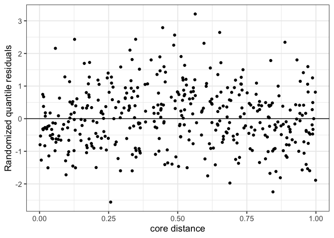
A plot of the residuals of the regression can also be generated using
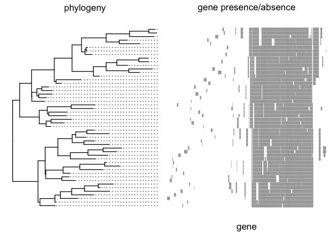
plot_residuals(fit_fast)A plot of the phylogeny and the corresponding gene presence/absence
matrix can be made using the plot_tree_pa function. This function also
takes an optional vector of gene names to include in the plot.
# look at only those genes that vary
variable_genes <- colnames(pa)[apply(pa, 2, sd) > 0]

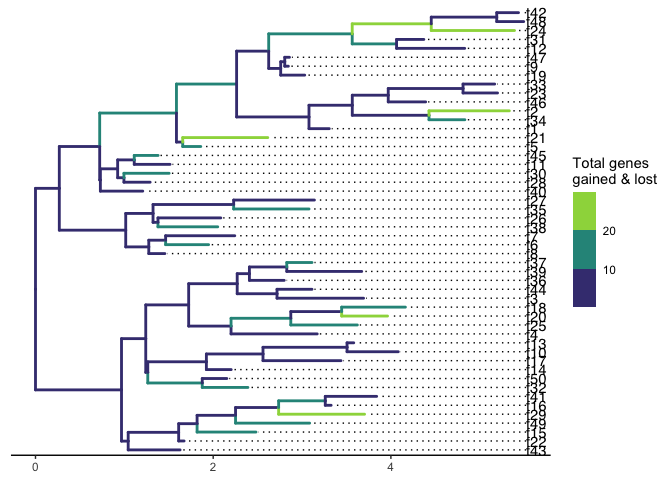
plot_tree_pa(tree = tree, pa = pa, genes = variable_genes, label_genes = FALSE, cols = "black")The plot_gain_loss function allows for the visualisation of the fitted
gene gain and loss events on the given phylogeny. The enrichment for
events at the tips of a tree is often driven by a combination of highly
mobile elements and annotation errors.
plot_gain_loss(fit)The tSNE dimension reduction technique can be used to investigate evidence for clusters within the pangenome.
plot_tsne(pa)The Mandrake method can also be used as an alternative to tSNE.
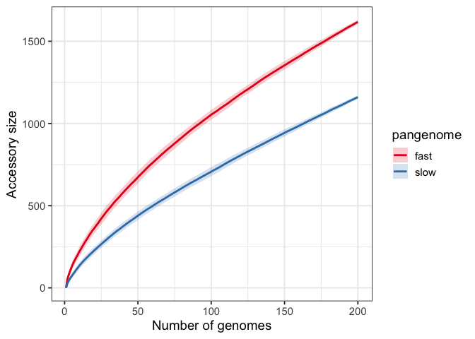
While we do not recommend the use of accumulation curves as they do not account for population structure, sampling bias or annotation errors we have included a function to plot them to make it easier for users to compare methods.
plot_acc(list(fast = sim_fast$pa, slow = sim_slow$pa))The name panstripe is an adaptation of ‘pinstripe’, the name of a long-nosed potoroo who was a villain in the playstation game Crash Bandicoot. The name was chosen as the program relies on the output of panaroo (named after the potoroo).

