package to create descriptive tables
- Overview
- News
- Package installation
- Costumizing the table
- Visual exploration
- Exporting the table
- Stratified tables
- Odds Ratios and Hazard Ratios
- Web-based User Interface
- Citation
compareGroups is an R package available on CRAN which performs
descriptive tables displaying means, standard deviation, quantiles or
frequencies of several variables. Also, p-value to test equality between
groups is computed using the appropiate test.
With a very simple code, nice, compact and ready-to-publish descriptives
table are displayed on R console. They can also be exported to different
formats, such as Word, Excel, PDF or inserted in a R-Sweave or
R-markdown document.
You will find an extensive manual describing all compareGropus
capabilities with real examples in the
vignette.
Also, compareGroups package has been published in Journal of Statistical Software [Subirana et al, 2014 http://www.jstatsoft.org/v57/i12/.].
Version 4.1
-
Compute confidence intervals of means, medians, proporcions or incidences
-
Proportions can be computed by rows as well as by columns, or by combinations of rows and columns (i.e. to sum up 100%).
-
New argument “position” to place tables justified to the left, centered or to the right using Rmarkdown.
-
When exporting tables to Excel,
export2xlsno longer usesxlsxpackage and useswrite_xlsxfunction from writexl pacakge, instead. -
The web-based user interface ,
cGroupsWUI(), has been improved and updated.
Version 4.0
-
New argument
var.equalto consider unequal variances when performing ANOVA tests. -
Date variables are supported.
-
New
strataTablefunction: to create stratified tables without having to use cbind. -
package vignette improved.
-
New
descrTablefunction that builds a descriptive table in one step. -
New options added in
export2md, to export tables in nicer format. -
New options added in
compareGroupsto control permutated chisquared test.
Install the compareGroups package from CRAN and then load it by
typing:
install.packages("compareGroups")
or from github to get the latest version
library(devtools)
devtools::install_github(repo = "isubirana/compareGroups")
In the following table, some variables from the PREDIMED study
(http://www.predimed.es/) are analysed. We illustrate the syntax of
compareGroups functions to display tables containing descriptives
or possible tests to compare groups.
Following, to describe all the variables of the data set just type:
library(compareGroups) # load compareGroups package
data(predimed) # load example data
descrTable(predimed)


--------Summary descriptives table ---------

__________________________________________________
                                    [ALL]      N
                                    N=6324
¯¯¯¯¯¯¯¯¯¯¯¯¯¯¯¯¯¯¯¯¯¯¯¯¯¯¯¯¯¯¯¯¯¯¯¯¯¯¯¯¯¯¯¯¯¯¯¯¯¯
Intervention group:                           6324
    Control                      2042 (32.3%)
    MedDiet + Nuts               2100 (33.2%)
    MedDiet + VOO                2182 (34.5%)
Sex:                                          6324
    Male                         2679 (42.4%)
    Female                       3645 (57.6%)
Age                              67.0 (6.17)  6324
Smoking:                                      6324
    Never                        3892 (61.5%)
    Current                      858 (13.6%)
    Former                       1574 (24.9%)
Body mass index                  30.0 (3.82)  6324
Waist circumference               100 (10.6)  6324
Waist-to-height ratio            0.63 (0.07)  6324
Hypertension:                                 6324
    No                           1089 (17.2%)
    Yes                          5235 (82.8%)
Type-2 diabetes:                              6324
    No                           3322 (52.5%)
    Yes                          3002 (47.5%)
Dyslipidemia:                                 6324
    No                           1746 (27.6%)
    Yes                          4578 (72.4%)
Family history of premature CHD:              6324
    No                           4895 (77.4%)
    Yes                          1429 (22.6%)
Hormone-replacement therapy:                  5661
    No                           5564 (98.3%)
    Yes                           97 (1.71%)
MeDiet Adherence score           8.68 (1.94)  6324
follow-up to main event (years)  4.36 (1.69)  6324
AMI, stroke, or CV Death:                     6324
    No                           6072 (96.0%)
    Yes                          252 (3.98%)
¯¯¯¯¯¯¯¯¯¯¯¯¯¯¯¯¯¯¯¯¯¯¯¯¯¯¯¯¯¯¯¯¯¯¯¯¯¯¯¯¯¯¯¯¯¯¯¯¯¯
Example
In the following table, variables are described by intervention group.
Some variables such as Waist-to-height ratio (wth) and MeDiet
Adherence score (p14) have been treated as non-normal distributed, and
medians and quantiles within square brackets instead of means and
standard deviations within round brackets are displayed. Also,
individuals older than 55 years old are selected. Appropiate tests to
compare means, medians or proportions are performed. For those binary
variables of type “yes/no”, you may desire to show only the proportion
of “yes” category without showing “yes” but only the variable name or
label. For example, for diabetes you may want to see simply “diabetes”
instead of “diabetes: yes”. This is possible by hide.no argument.
Note the simplicity of the syntax. Also, note the use of formula to
select the variables, and the use of subset to filter some individuals
as usual in many other R funcions.
tab <- descrTable(group ~ . , predimed, hide.no="no", method=c(wth=2, p14=2), subset=age>55)
tab


--------Summary descriptives table by 'group'---------

____________________________________________________________________________________________
                                    Control       MedDiet + Nuts   MedDiet + VOO   p.overall
                                     N=2001           N=2059           N=2141
¯¯¯¯¯¯¯¯¯¯¯¯¯¯¯¯¯¯¯¯¯¯¯¯¯¯¯¯¯¯¯¯¯¯¯¯¯¯¯¯¯¯¯¯¯¯¯¯¯¯¯¯¯¯¯¯¯¯¯¯¯¯¯¯¯¯¯¯¯¯¯¯¯¯¯¯¯¯¯¯¯¯¯¯¯¯¯¯¯¯¯¯
Sex:                                                                                <0.001
    Male                          780 (39.0%)      930 (45.2%)      865 (40.4%)
    Female                        1221 (61.0%)     1129 (54.8%)     1276 (59.6%)
Age                               67.6 (6.06)      66.9 (5.83)      67.3 (6.01)      0.001
Smoking:                                                                             0.490
    Never                         1268 (63.4%)     1250 (60.7%)     1340 (62.6%)
    Current                       255 (12.7%)      282 (13.7%)      272 (12.7%)
    Former                        478 (23.9%)      527 (25.6%)      529 (24.7%)
Body mass index                   30.3 (3.95)      29.7 (3.77)      29.9 (3.69)     <0.001
Waist circumference                101 (10.7)       100 (10.6)       100 (10.4)      0.024
Waist-to-height ratio           0.63 [0.59;0.68] 0.62 [0.58;0.67] 0.63 [0.58;0.67]  <0.001
Hypertension                      1683 (84.1%)     1709 (83.0%)     1753 (81.9%)     0.162
Type-2 diabetes                   950 (47.5%)      933 (45.3%)      1065 (49.7%)     0.016
Dyslipidemia                      1446 (72.3%)     1504 (73.0%)     1532 (71.6%)     0.559
Family history of premature CHD   454 (22.7%)      444 (21.6%)      501 (23.4%)      0.358
Hormone-replacement therapy        31 (1.71%)       30 (1.64%)       36 (1.87%)      0.854
MeDiet Adherence score          9.00 [7.00;10.0] 9.00 [8.00;10.0] 9.00 [8.00;10.0]  <0.001
follow-up to main event (years)   4.10 (1.74)      4.32 (1.70)      4.64 (1.59)     <0.001
AMI, stroke, or CV Death           95 (4.75%)       70 (3.40%)       84 (3.92%)      0.088
¯¯¯¯¯¯¯¯¯¯¯¯¯¯¯¯¯¯¯¯¯¯¯¯¯¯¯¯¯¯¯¯¯¯¯¯¯¯¯¯¯¯¯¯¯¯¯¯¯¯¯¯¯¯¯¯¯¯¯¯¯¯¯¯¯¯¯¯¯¯¯¯¯¯¯¯¯¯¯¯¯¯¯¯¯¯¯¯¯¯¯¯
Also, number of decimals and much more options can be changed to costumize the table as desired (see the package manual)
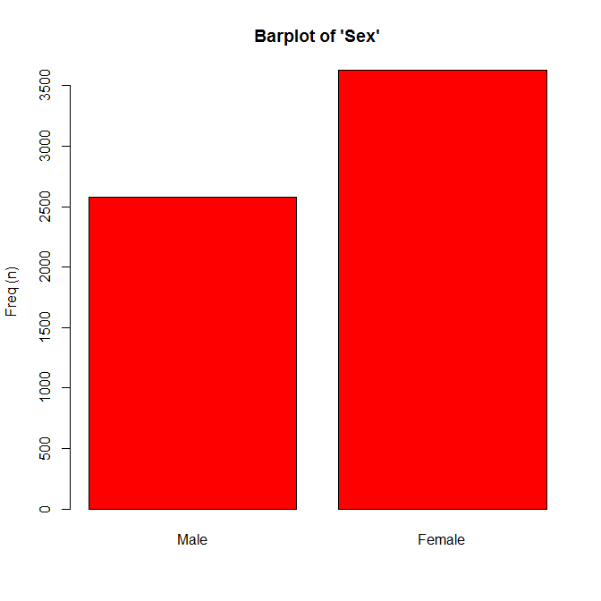
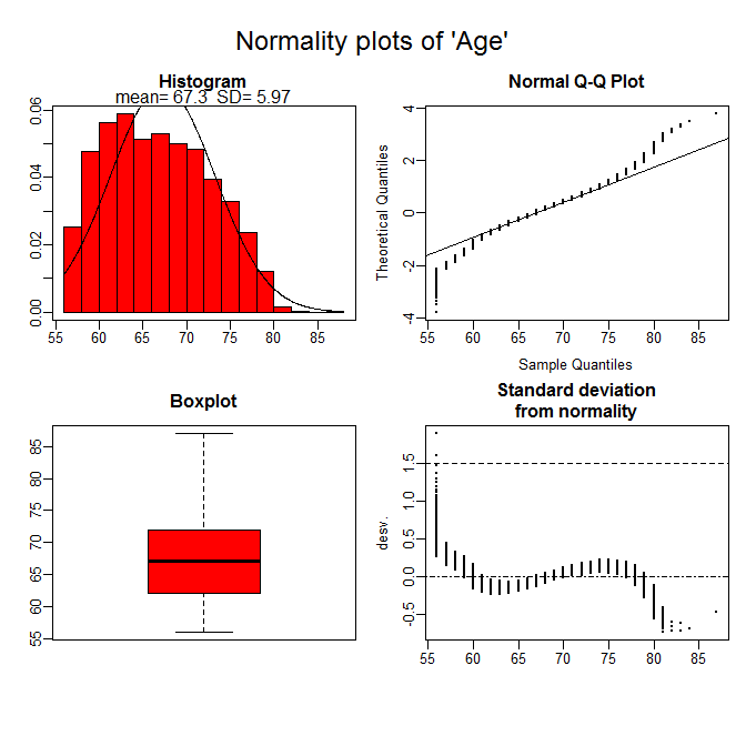
With compareGroups it is also possible to visualize the
distribution of analysed variables. This can be done by the plot
function applied on the table:
plot(tab["sex"]) # barplot
plot(tab["age"]) # histogram and normality plot
 |
 |
Once the table is created, it can be printed on the R console in a nice and compact format, or it can be exported to different formats, such as PDF, Excel, Word or LaTex code.
export2pdf(tab, file = "example.pdf")
export2xls(tab, file = "example.xlsx")
export2word(tab, file = "example.docx")
export2latex(tab, file = "example.tex")
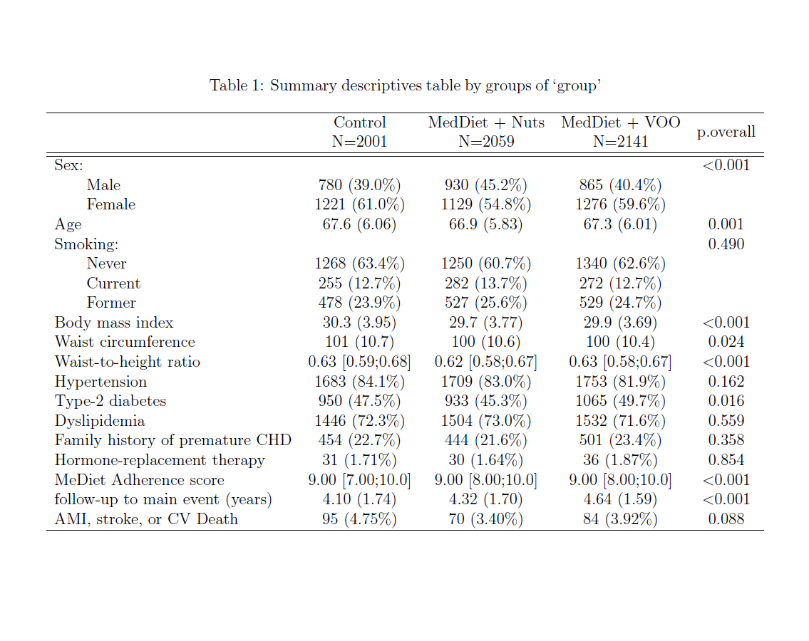
This is how the table looks like in PDF:
Also, by using export2md function a descriptive table can be inserted
in a Rmarkdown chunk to be compiled in HTML, PDF or Word report. Here
there is an example of a Rmarkdown compiled to HTML.
export2md(tab, strip = TRUE, first = TRUE,
          header.background = "blue", header.color = "white",
          caption = "Description of variables by intervention groups",
          size=10)
| Control | MedDiet + Nuts | MedDiet + VOO | p.overall | |
|---|---|---|---|---|
| N=2001 | N=2059 | N=2141 | ||
| Sex: | <0.001 | |||
| Male | 780 (39.0%) | 930 (45.2%) | 865 (40.4%) | |
| Female | 1221 (61.0%) | 1129 (54.8%) | 1276 (59.6%) | |
| Age | 67.6 (6.06) | 66.9 (5.83) | 67.3 (6.01) | 0.001 |
| Smoking: | 0.490 | |||
| Never | 1268 (63.4%) | 1250 (60.7%) | 1340 (62.6%) | |
| Current | 255 (12.7%) | 282 (13.7%) | 272 (12.7%) | |
| Former | 478 (23.9%) | 527 (25.6%) | 529 (24.7%) | |
| Body mass index | 30.3 (3.95) | 29.7 (3.77) | 29.9 (3.69) | <0.001 |
| Waist circumference | 101 (10.7) | 100 (10.6) | 100 (10.4) | 0.024 |
| Waist-to-height ratio | 0.63 \[0.59;0.68\] | 0.62 \[0.58;0.67\] | 0.63 \[0.58;0.67\] | <0.001 |
| Hypertension | 1683 (84.1%) | 1709 (83.0%) | 1753 (81.9%) | 0.162 |
| Type-2 diabetes | 950 (47.5%) | 933 (45.3%) | 1065 (49.7%) | 0.016 |
| Dyslipidemia | 1446 (72.3%) | 1504 (73.0%) | 1532 (71.6%) | 0.559 |
| Family history of premature CHD | 454 (22.7%) | 444 (21.6%) | 501 (23.4%) | 0.358 |
| Hormone-replacement therapy | 31 (1.71%) | 30 (1.64%) | 36 (1.87%) | 0.854 |
| MeDiet Adherence score | 9.00 \[7.00;10.0\] | 9.00 \[8.00;10.0\] | 9.00 \[8.00;10.0\] | <0.001 |
| follow-up to main event (years) | 4.10 (1.74) | 4.32 (1.70) | 4.64 (1.59) | <0.001 |
| AMI, stroke, or CV Death | 95 (4.75%) | 70 (3.40%) | 84 (3.92%) | 0.088 |
After creating a table you may want to repeat the descriptives within
stratas. For example, you may want to compare the groups for men and for
women. This is very easy using the strataTable function:
# stratify by sex
tabestr <- strataTable(tab, strata="sex")

# remove sex variable from the table
tabestr[-1]


--------Summary descriptives table ---------

__________________________________________________________________________________________________________________________________________________________
                                                            Male                                                         Female
                                ____________________________________________________________  ____________________________________________________________
                                    Control       MedDiet + Nuts   MedDiet + VOO   p.overall      Control       MedDiet + Nuts   MedDiet + VOO   p.overall
                                     N=780            N=930            N=865                       N=1221           N=1129           N=1276
¯¯¯¯¯¯¯¯¯¯¯¯¯¯¯¯¯¯¯¯¯¯¯¯¯¯¯¯¯¯¯¯¯¯¯¯¯¯¯¯¯¯¯¯¯¯¯¯¯¯¯¯¯¯¯¯¯¯¯¯¯¯¯¯¯¯¯¯¯¯¯¯¯¯¯¯¯¯¯¯¯¯¯¯¯¯¯¯¯¯¯¯¯¯¯¯¯¯¯¯¯¯¯¯¯¯¯¯¯¯¯¯¯¯¯¯¯¯¯¯¯¯¯¯¯¯¯¯¯¯¯¯¯¯¯¯¯¯¯¯¯¯¯¯¯¯¯¯¯¯¯¯¯¯
Age                               66.8 (6.32)      66.3 (6.10)      66.6 (6.31)      0.181      68.1 (5.84)      67.5 (5.54)      67.7 (5.75)      0.023
Smoking:                                                                             0.674                                                         0.923
    Never                         196 (25.1%)      259 (27.8%)      229 (26.5%)                 1072 (87.8%)     991 (87.8%)      1111 (87.1%)
    Current                       192 (24.6%)      229 (24.6%)      203 (23.5%)                  63 (5.16%)       53 (4.69%)       69 (5.41%)
    Former                        392 (50.3%)      442 (47.5%)      433 (50.1%)                  86 (7.04%)       85 (7.53%)       96 (7.52%)
Body mass index                   29.5 (3.46)      29.1 (3.27)      29.2 (3.24)      0.014      30.8 (4.18)      30.2 (4.07)      30.4 (3.90)      0.002
Waist circumference                104 (9.73)       103 (9.38)       103 (9.63)      0.251      99.1 (10.9)      97.8 (11.0)      98.0 (10.5)      0.009
Waist-to-height ratio           0.62 [0.58;0.65] 0.61 [0.58;0.65] 0.62 [0.58;0.65]   0.313    0.64 [0.60;0.69] 0.63 [0.58;0.68] 0.63 [0.59;0.68]   0.002
Hypertension                      626 (80.3%)      726 (78.1%)      656 (75.8%)      0.097      1057 (86.6%)     983 (87.1%)      1097 (86.0%)     0.733
Type-2 diabetes                   415 (53.2%)      480 (51.6%)      472 (54.6%)      0.455      535 (43.8%)      453 (40.1%)      593 (46.5%)      0.007
Dyslipidemia                      506 (64.9%)      621 (66.8%)      566 (65.4%)      0.691      940 (77.0%)      883 (78.2%)      966 (75.7%)      0.346
Family history of premature CHD   129 (16.5%)      157 (16.9%)      152 (17.6%)      0.849      325 (26.6%)      287 (25.4%)      349 (27.4%)      0.560
Hormone-replacement therapy        0 (0.00%)        0 (0.00%)        0 (0.00%)         .         31 (2.66%)       30 (2.82%)       36 (2.97%)      0.903
MeDiet Adherence score          9.00 [7.00;10.0] 9.00 [8.00;10.0] 9.00 [8.00;10.0]  <0.001    8.00 [7.00;10.0] 9.00 [8.00;10.0] 9.00 [7.00;10.0]  <0.001
follow-up to main event (years)   4.07 (1.79)      4.40 (1.73)      4.54 (1.64)     <0.001      4.12 (1.71)      4.26 (1.67)      4.72 (1.56)     <0.001
AMI, stroke, or CV Death           56 (7.18%)       41 (4.41%)       51 (5.90%)      0.048       39 (3.19%)       29 (2.57%)       33 (2.59%)      0.567
¯¯¯¯¯¯¯¯¯¯¯¯¯¯¯¯¯¯¯¯¯¯¯¯¯¯¯¯¯¯¯¯¯¯¯¯¯¯¯¯¯¯¯¯¯¯¯¯¯¯¯¯¯¯¯¯¯¯¯¯¯¯¯¯¯¯¯¯¯¯¯¯¯¯¯¯¯¯¯¯¯¯¯¯¯¯¯¯¯¯¯¯¯¯¯¯¯¯¯¯¯¯¯¯¯¯¯¯¯¯¯¯¯¯¯¯¯¯¯¯¯¯¯¯¯¯¯¯¯¯¯¯¯¯¯¯¯¯¯¯¯¯¯¯¯¯¯¯¯¯¯¯¯¯
or when is complied in HTML
export2md(tabestr, strip = TRUE, first = TRUE,
          header.background = "blue", header.color = "white", size=8)
|
|
Male |
Female |
||||||
|---|---|---|---|---|---|---|---|---|
| Control | MedDiet + Nuts | MedDiet + VOO | p.overall | Control | MedDiet + Nuts | MedDiet + VOO | p.overall | |
| N=780 | N=930 | N=865 | N=1221 | N=1129 | N=1276 | |||
| Sex: | . | . | ||||||
| Male | 780 (100%) | 930 (100%) | 865 (100%) | 0 (0.00%) | 0 (0.00%) | 0 (0.00%) | ||
| Female | 0 (0.00%) | 0 (0.00%) | 0 (0.00%) | 1221 (100%) | 1129 (100%) | 1276 (100%) | ||
| Age | 66.8 (6.32) | 66.3 (6.10) | 66.6 (6.31) | 0.181 | 68.1 (5.84) | 67.5 (5.54) | 67.7 (5.75) | 0.023 |
| Smoking: | 0.674 | 0.923 | ||||||
| Never | 196 (25.1%) | 259 (27.8%) | 229 (26.5%) | 1072 (87.8%) | 991 (87.8%) | 1111 (87.1%) | ||
| Current | 192 (24.6%) | 229 (24.6%) | 203 (23.5%) | 63 (5.16%) | 53 (4.69%) | 69 (5.41%) | ||
| Former | 392 (50.3%) | 442 (47.5%) | 433 (50.1%) | 86 (7.04%) | 85 (7.53%) | 96 (7.52%) | ||
| Body mass index | 29.5 (3.46) | 29.1 (3.27) | 29.2 (3.24) | 0.014 | 30.8 (4.18) | 30.2 (4.07) | 30.4 (3.90) | 0.002 |
| Waist circumference | 104 (9.73) | 103 (9.38) | 103 (9.63) | 0.251 | 99.1 (10.9) | 97.8 (11.0) | 98.0 (10.5) | 0.009 |
| Waist-to-height ratio | 0.62 \[0.58;0.65\] | 0.61 \[0.58;0.65\] | 0.62 \[0.58;0.65\] | 0.313 | 0.64 \[0.60;0.69\] | 0.63 \[0.58;0.68\] | 0.63 \[0.59;0.68\] | 0.002 |
| Hypertension | 626 (80.3%) | 726 (78.1%) | 656 (75.8%) | 0.097 | 1057 (86.6%) | 983 (87.1%) | 1097 (86.0%) | 0.733 |
| Type-2 diabetes | 415 (53.2%) | 480 (51.6%) | 472 (54.6%) | 0.455 | 535 (43.8%) | 453 (40.1%) | 593 (46.5%) | 0.007 |
| Dyslipidemia | 506 (64.9%) | 621 (66.8%) | 566 (65.4%) | 0.691 | 940 (77.0%) | 883 (78.2%) | 966 (75.7%) | 0.346 |
| Family history of premature CHD | 129 (16.5%) | 157 (16.9%) | 152 (17.6%) | 0.849 | 325 (26.6%) | 287 (25.4%) | 349 (27.4%) | 0.560 |
| Hormone-replacement therapy | 0 (0.00%) | 0 (0.00%) | 0 (0.00%) | . | 31 (2.66%) | 30 (2.82%) | 36 (2.97%) | 0.903 |
| MeDiet Adherence score | 9.00 \[7.00;10.0\] | 9.00 \[8.00;10.0\] | 9.00 \[8.00;10.0\] | <0.001 | 8.00 \[7.00;10.0\] | 9.00 \[8.00;10.0\] | 9.00 \[7.00;10.0\] | <0.001 |
| follow-up to main event (years) | 4.07 (1.79) | 4.40 (1.73) | 4.54 (1.64) | <0.001 | 4.12 (1.71) | 4.26 (1.67) | 4.72 (1.56) | <0.001 |
| AMI, stroke, or CV Death | 56 (7.18%) | 41 (4.41%) | 51 (5.90%) | 0.048 | 39 (3.19%) | 29 (2.57%) | 33 (2.59%) | 0.567 |
Using compareGroups package you can compute Odds Ratios for
transversal or case-control studies, or Hazard Ratios for cohort studies
- Example of case-control study: Odds Ratios
data(SNPs)
descrTable(casco ~ .-id, SNPs, show.ratio=TRUE, show.p.overall=FALSE)[1:4]


--------Summary descriptives table by 'casco'---------

_______________________________________________________________
                 0             1              OR        p.ratio
               N=47          N=110
¯¯¯¯¯¯¯¯¯¯¯¯¯¯¯¯¯¯¯¯¯¯¯¯¯¯¯¯¯¯¯¯¯¯¯¯¯¯¯¯¯¯¯¯¯¯¯¯¯¯¯¯¯¯¯¯¯¯¯¯¯¯¯
sex:
    Male    21 (44.7%)    54 (49.1%)         Ref.        Ref.
    Female  26 (55.3%)    56 (50.9%)   0.84 [0.42;1.67]  0.619
blood.pre   13.1 (0.88)   12.9 (1.03)  0.78 [0.55;1.11]  0.174
protein    39938 (19770) 44371 (24897) 1.00 [1.00;1.00]  0.280
snp10001:
    CC       2 (4.26%)    10 (9.09%)         Ref.        Ref.
    CT      21 (44.7%)    32 (29.1%)   0.33 [0.04;1.43]  0.147
    TT      24 (51.1%)    68 (61.8%)   0.60 [0.08;2.55]  0.521
¯¯¯¯¯¯¯¯¯¯¯¯¯¯¯¯¯¯¯¯¯¯¯¯¯¯¯¯¯¯¯¯¯¯¯¯¯¯¯¯¯¯¯¯¯¯¯¯¯¯¯¯¯¯¯¯¯¯¯¯¯¯¯
- Example of cohort study: Hazard Ratios
# create a Surv response:
library(survival)
predimed$tevent <- Surv(predimed$toevent, predimed$event=="Yes")

# perform descriptive table placing the Surv object as the response (left side of ~):
tab <- descrTable(tevent ~ .-toevent-event, predimed, method=c(wth=2,p14=2),
           hide.no="no", show.ratio=TRUE, show.p.overall=FALSE)

# print table on R console
print(tab, header.label=c("p.ratio"="p-value"))


--------Summary descriptives table by 'tevent'---------

__________________________________________________________________________________________
                                    No event          Event              HR        p-value
                                     N=6072           N=252
¯¯¯¯¯¯¯¯¯¯¯¯¯¯¯¯¯¯¯¯¯¯¯¯¯¯¯¯¯¯¯¯¯¯¯¯¯¯¯¯¯¯¯¯¯¯¯¯¯¯¯¯¯¯¯¯¯¯¯¯¯¯¯¯¯¯¯¯¯¯¯¯¯¯¯¯¯¯¯¯¯¯¯¯¯¯¯¯¯¯
Intervention group:
    Control                       1945 (32.0%)      97 (38.5%)          Ref.        Ref.
    MedDiet + Nuts                2030 (33.4%)      70 (27.8%)    0.66 [0.48;0.89]  0.008
    MedDiet + VOO                 2097 (34.5%)      85 (33.7%)    0.70 [0.53;0.94]  0.018
Sex:
    Male                          2528 (41.6%)     151 (59.9%)          Ref.        Ref.
    Female                        3544 (58.4%)     101 (40.1%)    0.49 [0.38;0.63] <0.001
Age                               66.9 (6.14)      69.4 (6.65)    1.06 [1.04;1.09] <0.001
Smoking:
    Never                         3778 (62.2%)     114 (45.2%)          Ref.        Ref.
    Current                       809 (13.3%)       49 (19.4%)    1.96 [1.40;2.74] <0.001
    Former                        1485 (24.5%)      89 (35.3%)    2.02 [1.53;2.67] <0.001
Body mass index                   30.0 (3.81)      29.8 (3.92)    0.99 [0.96;1.02]  0.455
Waist circumference                100 (10.6)       102 (10.6)    1.02 [1.01;1.03]  0.003
Waist-to-height ratio           0.63 [0.58;0.67] 0.63 [0.59;0.68] 5.27 [0.83;33.6]  0.079
Hypertension                      5025 (82.8%)     210 (83.3%)    1.10 [0.79;1.53]  0.578
Type-2 diabetes                   2841 (46.8%)     161 (63.9%)    1.88 [1.46;2.44] <0.001
Dyslipidemia                      4427 (72.9%)     151 (59.9%)    0.62 [0.49;0.80] <0.001
Family history of premature CHD   1378 (22.7%)      51 (20.2%)    0.93 [0.68;1.26]  0.640
Hormone-replacement therapy        96 (1.77%)       1 (0.45%)     0.29 [0.04;2.10]  0.223
MeDiet Adherence score          9.00 [7.00;10.0] 8.00 [7.00;10.0] 0.88 [0.83;0.94] <0.001
¯¯¯¯¯¯¯¯¯¯¯¯¯¯¯¯¯¯¯¯¯¯¯¯¯¯¯¯¯¯¯¯¯¯¯¯¯¯¯¯¯¯¯¯¯¯¯¯¯¯¯¯¯¯¯¯¯¯¯¯¯¯¯¯¯¯¯¯¯¯¯¯¯¯¯¯¯¯¯¯¯¯¯¯¯¯¯¯¯¯
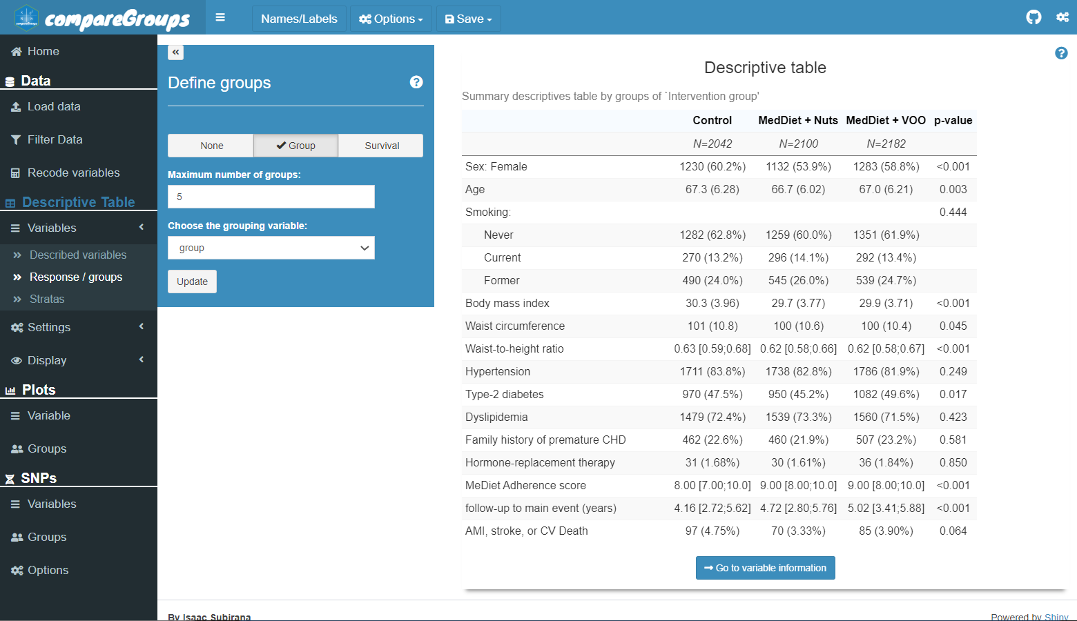
For those not familiar to R syntax, a Web User Interface (WUI) has been implemented using Shiny tools, which can be used remotely just accessing the compareGroups project website
Try the WUI compareGroups here
citation("compareGroups")


To cite compareGroups in publications use:

  Isaac Subirana, Hector Sanz, Joan Vila (2014). Building Bivariate
  Tables: The compareGroups Package for R. Journal of Statistical
  Software, 57(12), 1-16. URL https://www.jstatsoft.org/v57/i12/.

A BibTeX entry for LaTeX users is

  @Article{,
    title = {Building Bivariate Tables: The {compareGroups} Package for {R}},
    author = {Isaac Subirana and H\'ector Sanz and Joan Vila},
    journal = {Journal of Statistical Software},
    year = {2014},
    volume = {57},
    number = {12},
    pages = {1--16},
    url = {https://www.jstatsoft.org/v57/i12/},
  }
Subirana, Isaac, Héctor Sanz, and Joan Vila. 2014. “Building Bivariate Tables: The compareGroups Package for R.” Journal of Statistical Software 57 (12): 1–16. https://www.jstatsoft.org/v57/i12/.
