Overview of ‘personalized’

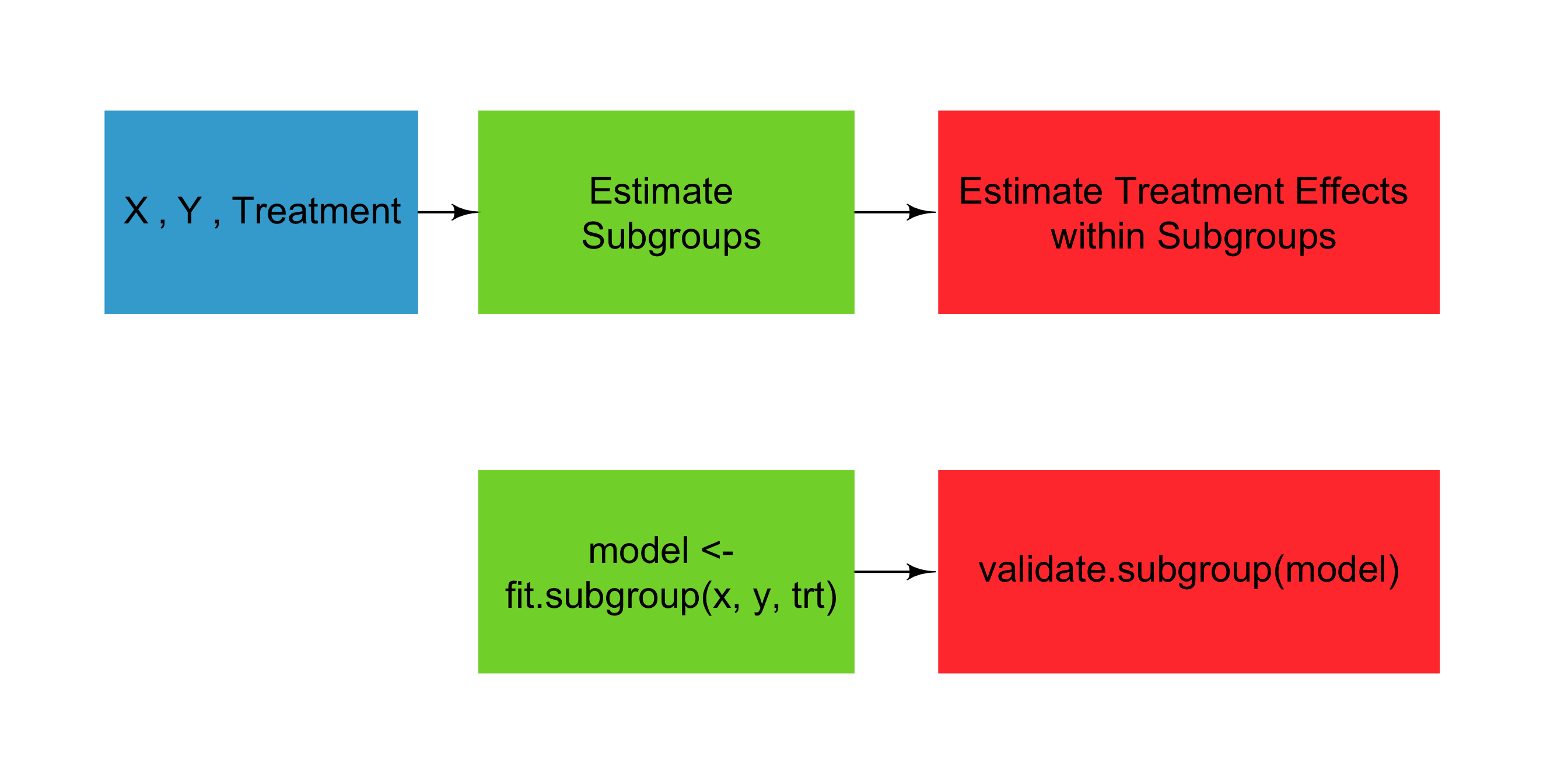
The ‘personalized’ package is designed for the analysis of data where the effect of a treatment or intervention may vary for different patients. It can be used for either data from randomized controlled trials or observational studies and is not limited specifically to the analysis of medical data.

The personalized package provides estimation methods for subgroup identification under the framework of Chen et al (2017). It also provides routines for valid estimation of the subgroup-specific treatment effects.

Documentation

Tutorial / Vignette
- tutorial of statistical methodology and usage of the package
Function help files

Installing the ‘personalized’ package

Install from CRAN using:

install.packages("personalized")

or install the development version using the devtools package:

devtools::install_github("jaredhuling/personalized")

or by cloning and building using R CMD INSTALL

Quick Usage Overview

Load the package:

library(personalized)

Create a propensity score model

(it should be a function which inputs covariates and treatments and returns propensity score):

prop.func <- function(x, trt)
{
    # fit propensity score model
    propens.model <- cv.glmnet(y = trt,
                               x = x, family = "binomial")
    pi.x <- predict(propens.model, s = "lambda.min",
                    newx = x, type = "response")[,1]
    pi.x
}

Fit a model to estimate subgroup:

subgrp.model <- fit.subgroup(x = x, y = y,
                             trt = trt,
                             propensity.func = prop.func,
                             loss   = "sq_loss_lasso",
                             nfolds = 5)              # option for cv.glmnet

Display estimated subgroups and variables selected which determine the subgroups:

summary(subgrp.model)

## family:    gaussian 
## loss:      sq_loss_lasso 
## method:    weighting 
## cutpoint:  0 
## propensity 
## function:  propensity.func 
## 
## benefit score: f(x), 
## Trt recom = Trt*I(f(x)>c)+Ctrl*I(f(x)<=c) where c is 'cutpoint'
## 
## Average Outcomes:
##                Recommended Ctrl    Recommended Trt
## Received Ctrl -3.9319 (n = 109) -21.2055 (n = 122)
## Received Trt  -25.078 (n = 112)   -8.326 (n = 157)
## 
## Treatment effects conditional on subgroups:
## Est of E[Y|T=Ctrl,Recom=Ctrl]-E[Y|T=/=Ctrl,Recom=Ctrl] 
##                                      21.1461 (n = 221) 
##     Est of E[Y|T=Trt,Recom=Trt]-E[Y|T=/=Trt,Recom=Trt] 
##                                      12.8795 (n = 279) 
## 
## NOTE: The above average outcomes are biased estimates of
##       the expected outcomes conditional on subgroups. 
##       Use 'validate.subgroup()' to obtain unbiased estimates.
## 
## ---------------------------------------------------
## 
## Benefit score quantiles (f(X) for Trt vs Ctrl): 
##      0%     25%     50%     75%    100% 
## -9.2792 -1.8237  0.5011  2.5977  9.6376 
## 
## ---------------------------------------------------
## 
## Summary of individual treatment effects: 
## E[Y|T=Trt, X] - E[Y|T=Ctrl, X]
## 
##     Min.  1st Qu.   Median     Mean  3rd Qu.     Max. 
## -18.5583  -3.6474   1.0023   0.9507   5.1954  19.2753 
## 
## ---------------------------------------------------
## 
## 5 out of 50 interactions selected in total by the lasso (cross validation criterion).
## 
## The first estimate is the treatment main effect, which is always selected. 
## Any other variables selected represent treatment-covariate interactions.
## 
##             Trt     V2     V11     V17    V32    V35
## Estimate 0.5463 0.9827 -0.4356 -0.1532 0.0326 0.1007

Use repeated train and test splitting to estimate subgroup treatment effects:

val.model <- validate.subgroup(subgrp.model, B = 100,
                               method = "training_test",
                               train.fraction = 0.75)

Display estimated subgroup treatment effects:

print(val.model, digits = 2, sample.pct = TRUE)

## family:  gaussian 
## loss:    sq_loss_lasso 
## method:  weighting 
## 
## validation method:  training_test_replication 
## cutpoint:           0 
## replications:       100 
## 
## benefit score: f(x), 
## Trt recom = Trt*I(f(x)>c)+Ctrl*I(f(x)<=c) where c is 'cutpoint'
## 
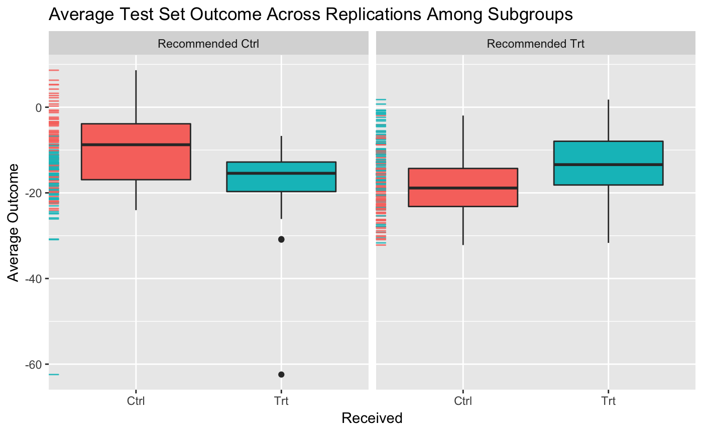
## Average Test Set Outcomes:
##                         Recommended Ctrl           Recommended Trt
## Received Ctrl  -9.56 (SE = 7.98, 19.88%) -18.62 (SE = 6.72, 26.5%)
## Received Trt  -16.64 (SE = 6.85, 23.23%) -13.41 (SE = 7.8, 30.39%)
## 
## Treatment effects conditional on subgroups:
## Est of E[Y|T=Ctrl,Recom=Ctrl]-E[Y|T=/=Ctrl,Recom=Ctrl] 
##                              6.54 (SE = 10.49, 43.11%) 
##     Est of E[Y|T=Trt,Recom=Trt]-E[Y|T=/=Trt,Recom=Trt] 
##                              5.21 (SE = 11.06, 56.89%) 
## 
## Est of 
## E[Y|Trt received = Trt recom] - E[Y|Trt received =/= Trt recom]:                 
## 2.91 (SE = 8.29)

Visualize subgroup-specific treatment effect estimates across training/testing iterations:

plot(val.model)

Investigate the marginal characteristics of the two estimated subgroups

Here we only display covariates with a significantly different mean value (at level 0.05)

summ <- summarize.subgroups(subgrp.model)
print(summ, p.value = 0.05)

##     Avg (recom Ctrl) Avg (recom Trt) Ctrl - Trt SE (recom Ctrl)
## V2           -2.4161          1.9013     -4.317          0.1423
## V11           1.1279         -0.7963      1.924          0.1914
## V17           0.8053         -0.3715      1.177          0.2170
##     SE (recom Trt)
## V2          0.1298
## V11         0.1572
## V17         0.1736

Accessing Help Files for Main Functions of `personalized`

Access help files for the main functions of the personalized package:

?fit.subgroup
?validate.subgroup