Abeshu et al., 2023, GMD

Enhancing the representation of water management in global hydrological models

Guta Wakbulcho Abeshu¹, Fuqiang Tian², Thomas Wild³, Mengqi Zhao⁴, Sean Turner³, A F M Kamal Chowdhury⁵, Chris R. Vernon⁴, Hongchang Hu², Yuan Zhuang², Mohamad Hejazi³⁺ and Hong-Yi Li1^1*
¹ Department of Civil and Environmental Engineering, University of Houston, Houston, 77204, US
² Department of Hydraulic Engineering, Tsinghua University, Beijing, 100084, China
³ Joint Global Change Research Institute, Pacific Northwest National Laboratory, College Park, MD 20740, US
⁴ Pacific Northwest National Laboratory, Richland, WA 99354, US
⁵ Earth System Science Interdisciplinary Center (ESSIC), University of Maryland, College Park, MD 20740, US

+ Now at King Abdullah Petroleum Studies and Research Center (KAPSARC), Riyadh, Saudi Arabia
* corresponding author: hongyili.jadison@gmail.com

Abstract

This study enhances an existing global hydrological model (GHM), Xanthos, by adding a new water management module that distinguishes between the operational characteristics of irrigation, hydropower, and flood control reservoirs. We remapped reservoirs in the GranD database to Xanthos' 0.5-degree spatial resolution so that a single lumped reservoir exists per grid cell, which yielded 3790 large reservoirs. We implemented unique operation rules for each reservoir type based on their primary purposes. In particular, hydropower reservoirs have been treated as flood control reservoirs in previous GHM studies, while here, we determined the operation rules for hydropower reservoirs via optimization that maximizes long-term hydropower production. We conducted global simulations using the enhanced Xanthos and validated monthly streamflow for 91 large river basins where high-quality observed streamflow data were available. A total of 1878 (296 hydropower, 486 irrigation, and 1096 flood control and others) out of the 3790 reservoirs are located in the 91 basins and are part of our reported results. The Kling-Gupta Efficient (KGE) value (after adding the new water management) is ≥ 0.5 and ≥ 0.0 in 39 and 81 basins, respectively. After adding the new water management module, model performance improved for 75 out of 91 basins and worsened for only seven. To measure the relative difference between explicitly representing hydropower reservoirs and representing hydropower reservoirs as flood control reservoirs (as is commonly done in other GHMs), we use normalized-root-mean-square-error (NRMSE) and the coefficient of determination (R2). Out of the 296 hydropower reservoirs, NRMSE is > 0.25 (i.e., considering 0.25 to represent a moderate difference) for over 44% of the 296 reservoirs when comparing both the simulated reservoir releases and storage time series between the two simulations. We suggest that correctly representing hydropower reservoirs in GHMs could have important implications for our understanding and management of freshwater resource challenges at regional-to-global scales. This enhanced global water management modeling framework will allow for the analysis of future global reservoir development and management from a coupled human-earth system perspective.

Journal reference

Abeshu, G.W., Tian, F., Wild, T., Zhao, M., Sean Turner, Chowdhury, K., Vernon, C., Hu, H., Zhuang, Y., Hejazi, M., and Li, H., Enhancing the representation of water management in global hydrological models. GMD

Code reference

The model used in this manuscript can be found at https://github.com/gutabeshu/xanthos-wm

Data reference

Input data

The following are input data required to run the model

Forcing Data: In the study, we used gridded climatic data from the WATer and global CHange (WATCH; Weedon et al., 2011) dataset from 1971 to 2001. The global monthly datasets include precipitation, maximum temperature, relative humidity and minimum temperature. DataHub: https://www.isimip.org/gettingstarted/input-data-bias-adjustment/details/3/
Water demand and water use data: Monthly water demand and consumptive water use data for various sectors at a 0.5-degree resolution are from Huang et al. (2018), which are available from 1971 to 2010. DataHub: https://doi.org/10.5281/zenodo.1209296
Reservoirs Data: Global reservoir data are obtained from the GRanD dataset (Lehner et al., 2011). The GRanD database we use here only considers reservoirs with storage capacity values greater than 0.1 km3. Reservoirs with missing storage capacity and those identified with purposes such as tide control are dropped, reducing the total GranD reservoirs from 6862 to 6847. DataHub: https://doi.org/10.7927/H4HH6H08
Streamflow Data: Observed stream flow data for model parameter identification and validation are obtained from the Global Runoff Data Center (GRDC)DataHub: https://www.bafg.de/GRDC

Output data

Xanthos-WM output dataset name. DataHub: https://doi.org/10.5281/zenodo.7557403

Contributing modeling software

Model	Version	Repository Link	DOI
Xanthos	version	https://github.com/gutabeshu/xanthos-wm steps for installation can be found at https://github.com/JGCRI/xanthos	https://doi.org/10.5281/zenodo.7557380

Reproduce my experiment

Get xanthos-wm from https://github.com/gutabeshu/xanthos-wm
Install the software components required to conduct the experiment from Contributing modeling software
Download the supporting input data required to conduct the experiment from https://doi.org/10.5281/zenodo.7557403. The input data folder is labeled 'example', place it in the 'xanthos-wm' folder and unzip.
Under xanthos-wm find 'pm_abcd_mrtm_managed.ini' and date the following as needed:
- 'basin_list = 229, 230, 231':provide list of IDs of basins you would like to run (IDs of CONUS basins are 7, 217 - 226, 228, 230, 233)
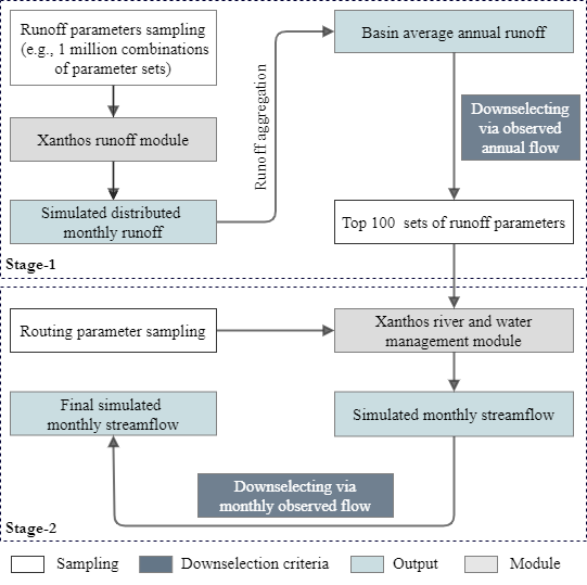
- 'set_calibrate=1': If the basin is in CONUS this will automatically perform both the Stage-1 and Stage-2 calibration process shown below
After the run is complete the calibration process and model output can be found under 'xanthos-wm/example/output'

Script Name	Description	How to Run
`Figure-X.py`	Script to compare my outputs to the original	edit the `dir_in` at the beginning to your output directory

File Modification
Modify every directory within this file(Files to be modified) to the directory that holds your required input data to run the model.

Model	Programming Language	Files to be Modified
Xanthos	Python 3.3+	xanthos-wm/pm_abcd_mrtm_managed.ini

Reproduce my figures

Use the scripts found in the figures directory to reproduce the figures used in this publication.

Get the model output data from your simulation or can be obtained from https://doi.org/10.5281/zenodo.7557403. The output data folder is labeled 'Data for Figures-Xanthos WM'
Open the 'Figure-X.ipyn' you would like to reproduce
Update directories for input data (i.e., model outputs) and figure output at the beginning
Run the script corresponding to the figure of interest.

Script Name	Description	How to Run
`Figure_1.drawio`	Sketch to generate Figure 1	`Figure_1.drawio` opens on drawio
`Figure_2.drawio`	Sketch to generate Figure 2	`Figure_2.drawio` opens on drawio
`Figure_3.ipynb`	Script to generate Figure 3	`Figure_3.ipynb change input/output directory path` & run on notebook
`Figure_4.ipynb`	Script to generate Figure 4	`Figure_4.ipynb change input/output directory path` & run on notebook
`Figure_5.ipynb`	Script to generate Figure 5	`Figure_5.ipynb change input/output directory path` & run on notebook
`Figure_6.ipynb`	Script to generate Figure 6	`Figure_6.ipynb change input/output directory path` & run on notebook
`Figure_7.ipynb`	Script to generate Figure 7	`Figure_7.ipynb change input/output directory path` & run on notebook
`Figure_8.ipynb`	Script to generate Figure 8	`Figure_8.ipynb change input/output directory path` & run on notebook
`Figure_9.ipynb`	Script to generate Figure 9	`Figure_9.ipynb change input/output directory path` & run on notebook
`Figure_S1.ipynb`	Script to generate Figure S1	`Figure_S1.ipynb change input/output directory path` & run on notebook
`Figure_S2.ipynb`	Script to generate Figure S2	`Figure_S2.ipynb change input/output directory path` & run on notebook
`Figure_S3.ipynb`	Script to generate Figure S3	`Figure_S3.ipynb change input/output directory path` & run on notebook
`Figure_S4.ipynb`	Script to generate Figure S4	`Figure_S4.ipynb change input/output directory path` & run on notebook
`Figure_S5.ipynb`	Script to generate Figure S5	`Figure_S5.ipynb change input/output directory path` & run on notebook
`Figure_S6.ipynb`	Script to generate Figure S6	`Figure_S6.ipynb change input/output directory path` & run on notebook

gutabeshu/Abeshu-etal_2023_GMD