Scripts and figures accompanying Diverse Primary and Secondary Structural Features Are Associated With Y Complex-Dependent mRNA Maturation in Bacillus subtilis
Below you will find detailed instructions for recreating each figure/means of analysis presented in the paper. If you have questions that are beyond the scope of the paper or this repository [e.g. technical questions like "What shell commands and scripts would I need to run to grab sequence windows for all 21 sites?"] please contact me.
Please note that all figures used in the paper can also be found under figures/. All varna files for structures can be found under varna/.
###Quick note on bedtools getfasta
Bedtools getfasta will not reverse complement strands for you. Please take your getfasta output and corresponding bedfile and use as input to strand_directionality.py. Note that this script needs base_complement.py and string_reversal.py to run, so keep those in the same directory.
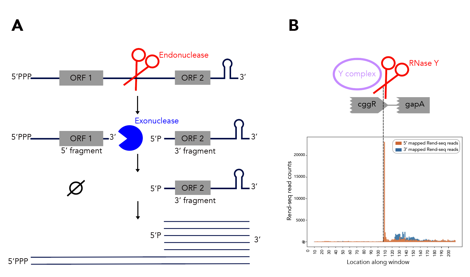
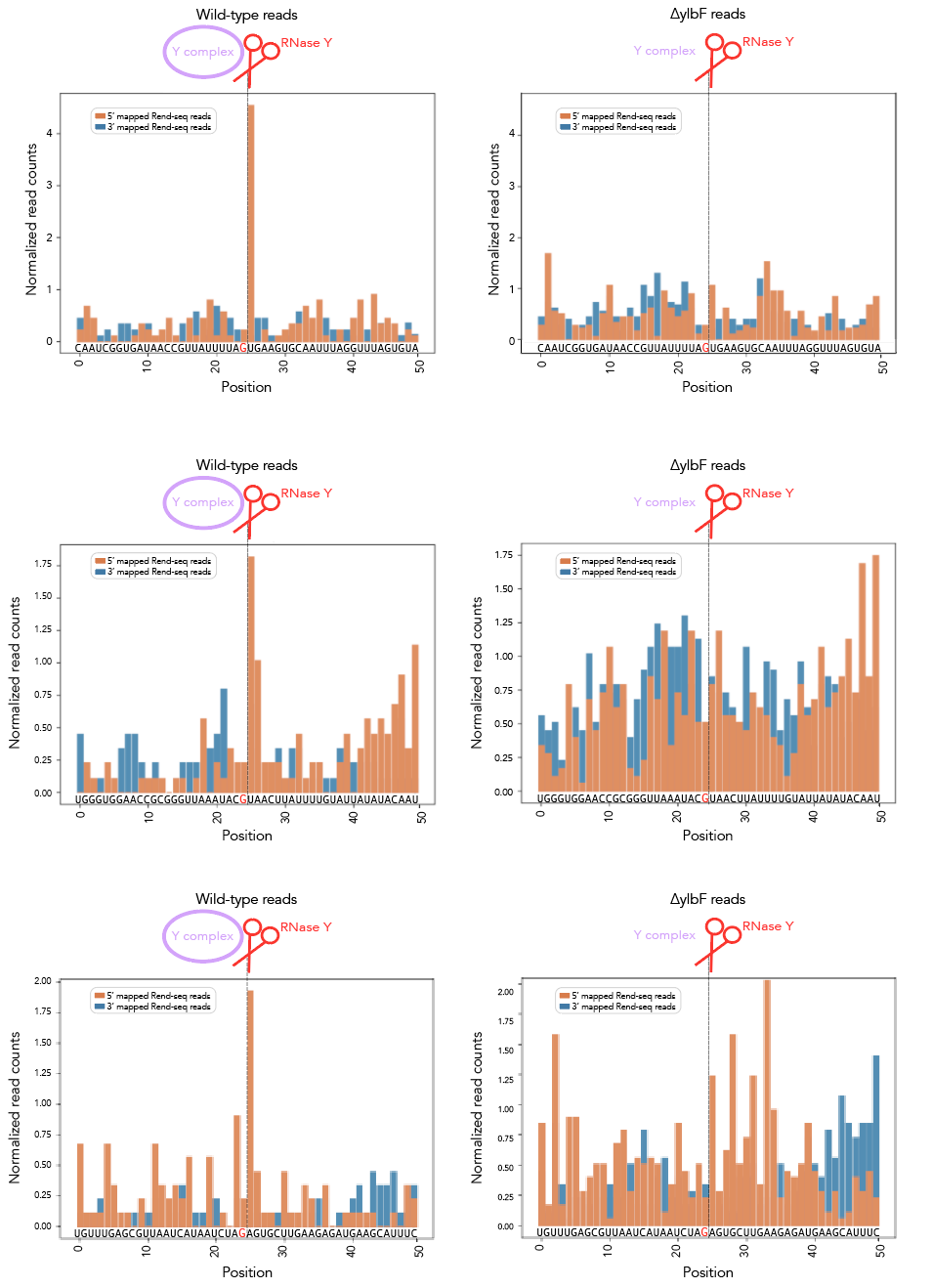
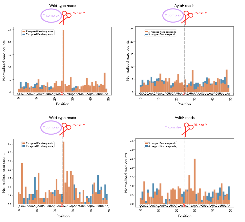
Should you want rend-seq visualizations of the 200nt windows I've been using, look no further than rend_seq/. I've included the following wigs [all libraries prepared from cells in LB exponential]:
- WT B. subtilis 168 ["wt*"]
- ∆RNase J1 168 ["rnj*"]
- 168 treated with a 5' exonuclease to identify 5' monophosphates [to determine if a 5' end is an alternative isoform or the product of cleavage] ["5exo*"]
- ∆PNPase 168 [to identify 3' peaks that may result from cleavage] ["pnpA*"]
- ∆RNase Y 168 ["rny*"]
- ∆ ylbF 168 ["ylbF*"]
Add the appropriate 5'f/r and 3'f/r wigs into rend_seq/plot_rend_seq.py [currently can only plot one set of 5'/3/ files but it's a really easy fix to modify if needed] and run! If you want to visualize a different set of windows, just use a different bedfile as input--21_cleavage_final.bed12 contains all 21 windows that I use for analysis. You can verify these sequences in Mochiview if you'd like--go to mochiview/subtilis_mochiview. There are wigs for [all using derivatives of B. subtilis strain 168 in LB exponential] wt, ∆RNase Y, ∆_ylbF_, ∆_yaaT_ and ∆_ymcA_. You can use Mochiview's find function to search for the 200nt windows, i.e. 21_cleavage_final.txt.
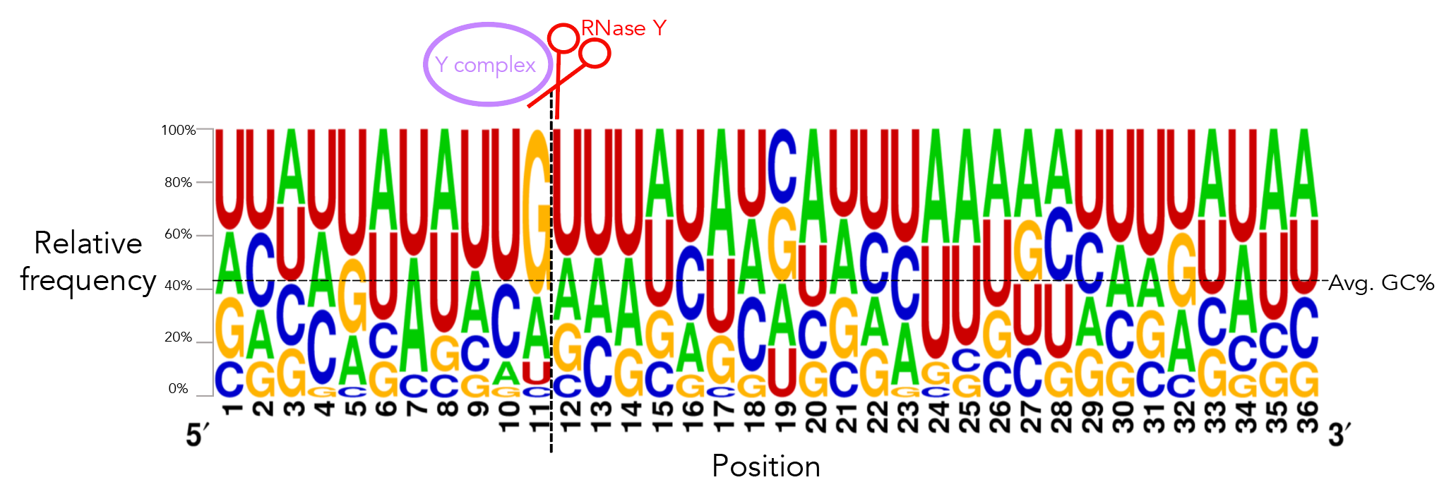
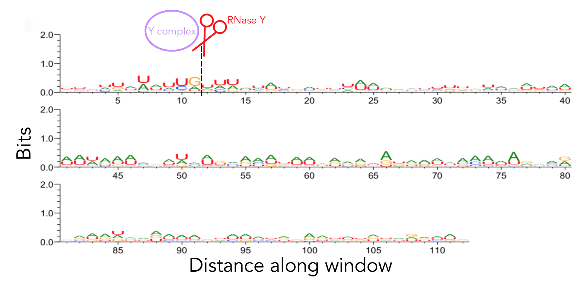
To recreate figure 2-2 use seqlogo/rna_21_cleavage_for_seqlogo.txt [This is a fasta-format file containing RNA sequences of all 21 windows used. I've shortened my windows from the original ~200nt for visualization purposes so each window contains 25nt after the cleavage site. Since not all windows contain 25nt before the cleavage site I've standardized the length of all windows to be that of the shortest window, meaning that there are 12nt before the cleavage site. Please see methods if the rationale behind this is confusing. For figure S12 use seqlogo/rna_shortened_21_cleavage_final.txt. In both instances all cleavage sites occur between one-indexed nucleotides 11 and 12] as an input to weblogo, making sure to click the "Frequency Plot" option. You can view the full 112nt window used for frequency plot analysis using rna_shortened_21_cleavage_final.txt.
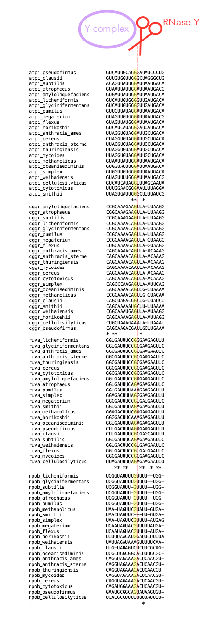
I use Clustalw2 in shell to run all my MSAs. Under msa/ I have directories for each cleavage site producing a MSA with alignment-to-subtilis score >30. The actual alignment is provided in each subdirectory as a *.aln file. I've included alignments for all other sites for which I found sufficient homologs to construct a MSA under msa/msas_with_bad_scores. All genomes are available under genome_fasta_files/ [this also has a file for the staph genome]. I first grab sequences from my fasta files [atpi_correct_evolutionary.txt], standardize the length of all sequences to be that of the shortest sequences [equal_size_sequences_seqlogo.py] and convert all T's to U's [dna_to_rna_sequences.py]. From there I run the MSA on my equal-length RNA sequences [rna_atpi_correct_evolutionary.txt] using the slow/accurate option. If you want to further shorten sequences to visualize their sequence logos I've included shorten_for_seqlogo.py--this produces 50nt windows that you can use in weblogo. That's really more for fun, though. Those sequence logos don't really tell you much. Unfortunately there's no way to denote the cleavage site in the MSA itself so you have to search for it manually.
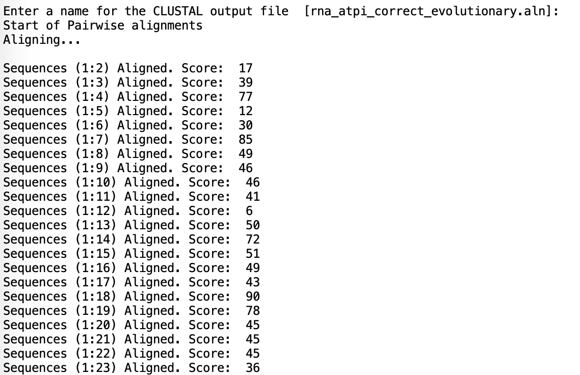
If you want to recalculate the alignment-to-subtilis scores, take the average of all pairwise alignment scores of the form "Sequences (1:n) Aligned. Score: " [as seen above]. Note that ClustalW2 will output these scores prior to producing the MSA, so be on the lookout. Sequence 1 in all *_evolutionary.txt files is always the subtilis sequence. This was easy enough to do manually that I didn't bother automating it.
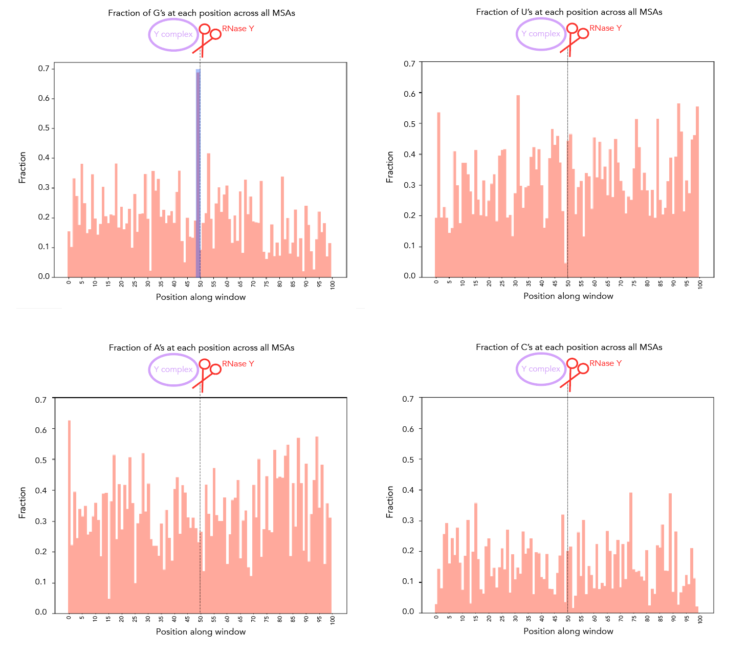
Shortened MSA snippets around the cleavage site [50nt either side] are under msa/msa_nucleotide_enrichment/*.txt. sequences_for_analysis.txt contains all 8 MSAs, whereas the other *.txt files are for individual MSAs. You can check for enrichment of A/U/C/G by running plots_of_sequences.py and adding the appropriate file as input. I didn't find looking at individual MSAs to be particularly illuminating but I've included them in here regardless.
Use staph/staph_rny_sites.txt as input into weblogo, making sure to click the "Frequency Plot" option.
Run staph/values_from_rend_seq_staph.py. I'm only plotting the 5 seemingly Y complex-dependent sites. The sixth one corresponds to the sequence TACTTACTAAATTTTATTTAACCTAAAAATGAACCACCTGGATGTGTGGG and doesn't seem to be Y complex-dependent. The locations of all staph cleavage sites from this paper can be found in staph/staph_rny_sites.txt. The wig files under staph/ need slight modification to run in mochiview. If this is your goal, go to mochiview/staph_mochiview/. There you can find wt and ∆rny data for our staph strain [wt files are under wt* and ∆ylbF are under ylbF*]. We map reads to the NC_007795 genome. You can grab the NC_007795 cds from the NCBI site here. This requires some modification to be converted to the Mochiview format, so you can use staph_mochiview/convert_mochiview_location.py to do the conversion for you. Or you can just use the already-converted CDS I have, namely NC_007795_mochi_cds.txt. The one benefit of using the script is that it should work for any CDS that needs conversion from NCBI->Mochiview, not just NC_007795.
I ran weblogo in shell for this--the input file for figure 2-6 is seqlogo/rna_21_cleavage_for_seqlogo.txt [output available in seqlogo/sequence_logo.eps] and the input for figure S13 is seqlogo/rna_shortened_21_cleavage_final.txt. The output file is seqlogo/sequence_logo.eps. The seqlogo directory also has other files that can be used as input--rna*.txt files have AUCG sequences whereas others have ATCG. To produce rna_21_cleavage_for_seqlogo.txt I took 21_cleavage_final.txt, ran equal_size_sequences_seqlogo.py to standardize the length of all input sequences to be that of the shortest sequences and then ran shorten_for_seqlogo.py to get at most a 50nt window. I realize that equal_size_sequences_seqlogo.py and shorten_for_seqlogo.py are somewhat redundant scripts. shorten_for_seqlogo.py will honestly get the job done if you're ok hard-coding window sizes.
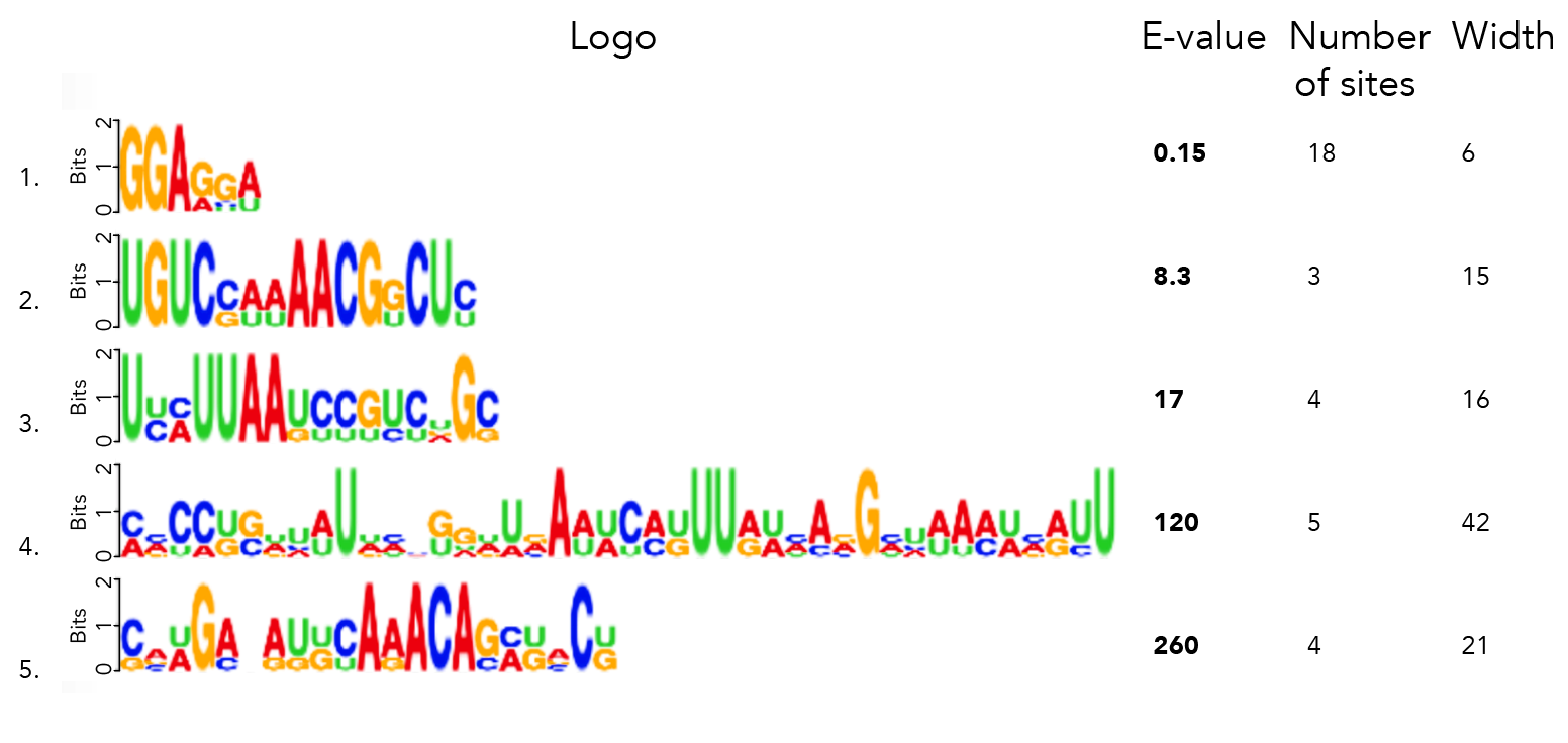
I ran MEME on 21_cleavage_final.txt to find the top 5 motifs with a minimum motif width of 3nt and max width of 50nt. Running the search with both a 0-order and 1st-order background yields the same results.
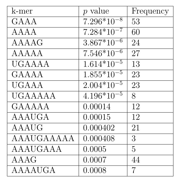
For this I ran kmer_analysis/kmer_distribution.py. This prints out a list of all k-mers in ascending order of p value. For each k-mer I also note the number of times it appeared in the 21 sites. To get the probabilities of A/U/G/C I ran kmer_analysis/nt_probabilities.py.
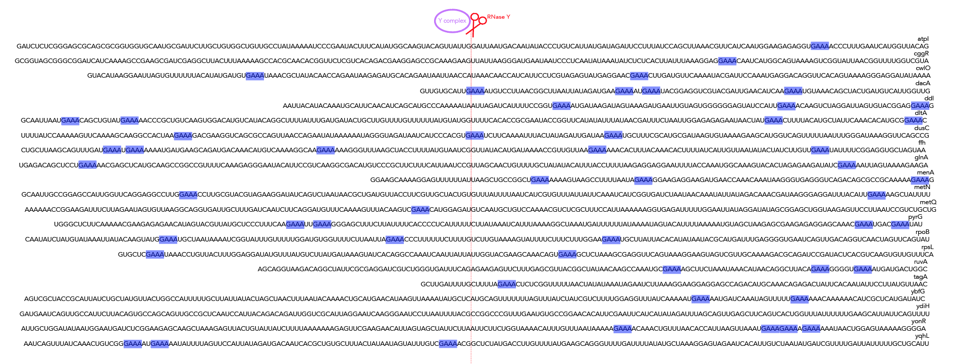
For these figures I literally just searched through the sequences and found the matching k-mers. Nothing fancy.
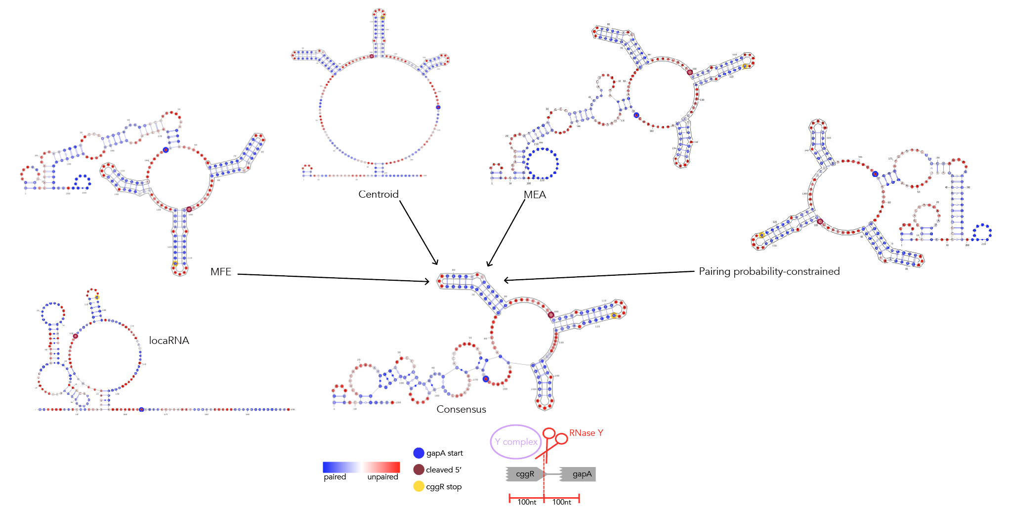
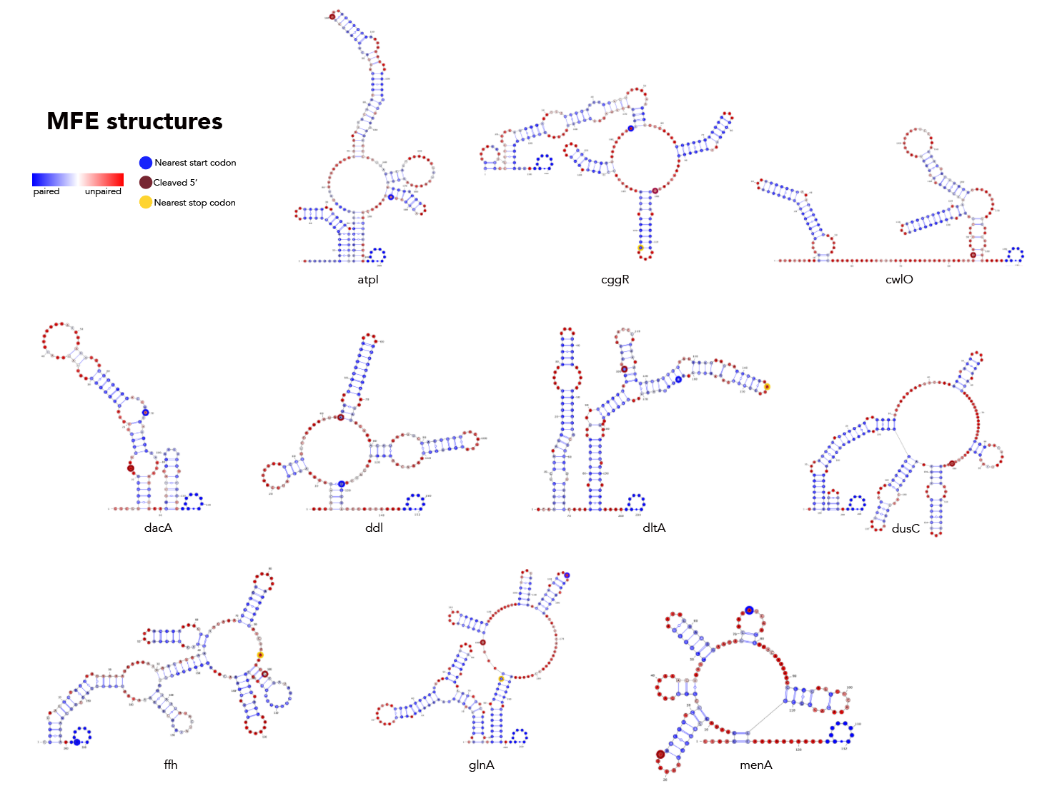
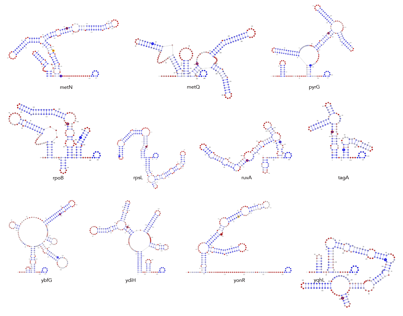
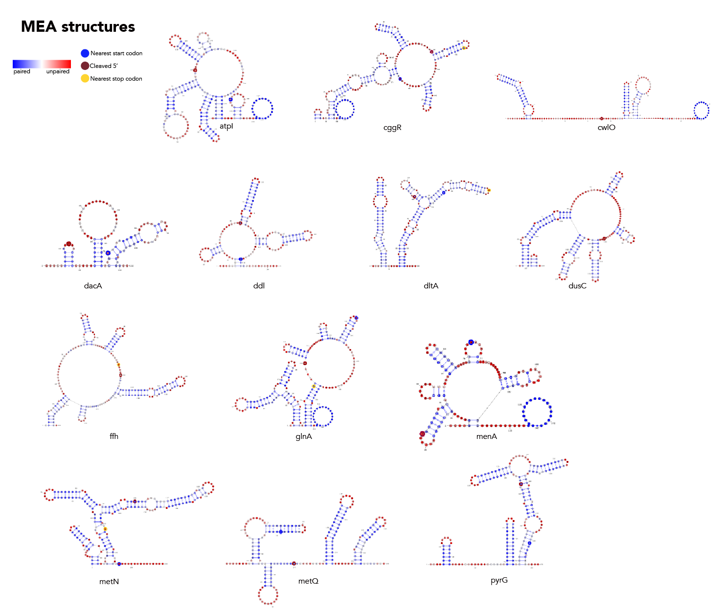
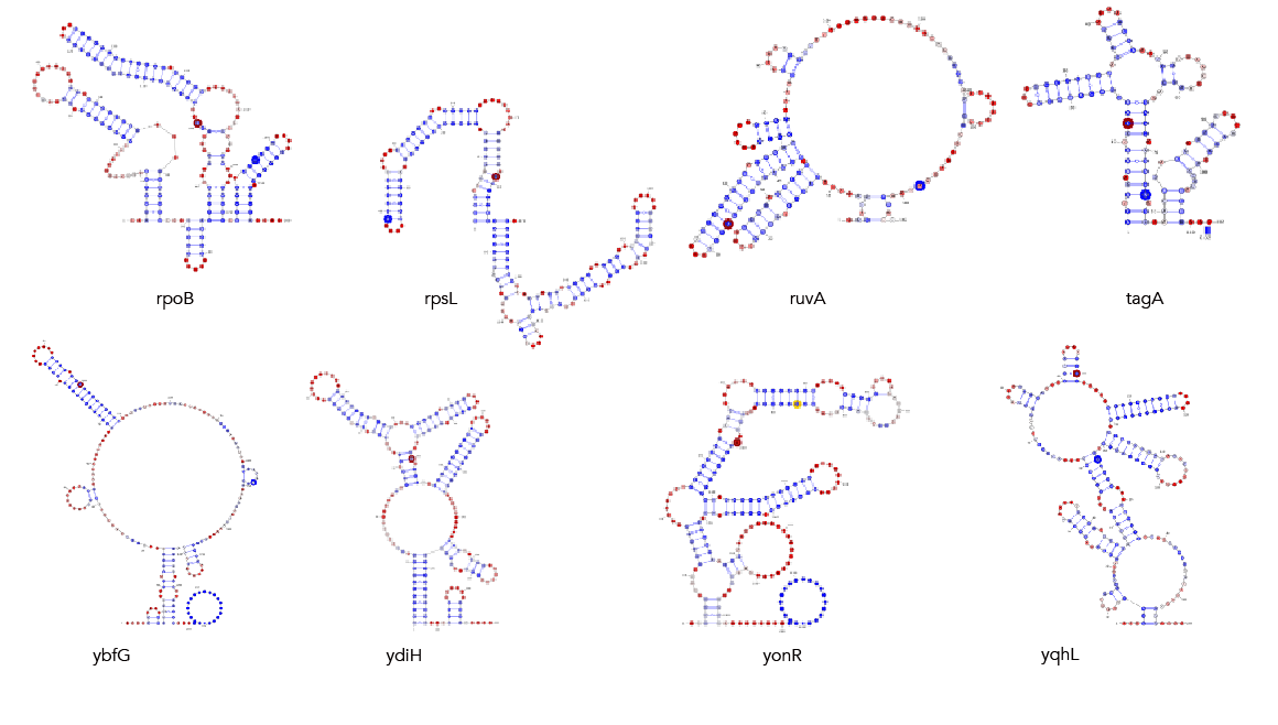
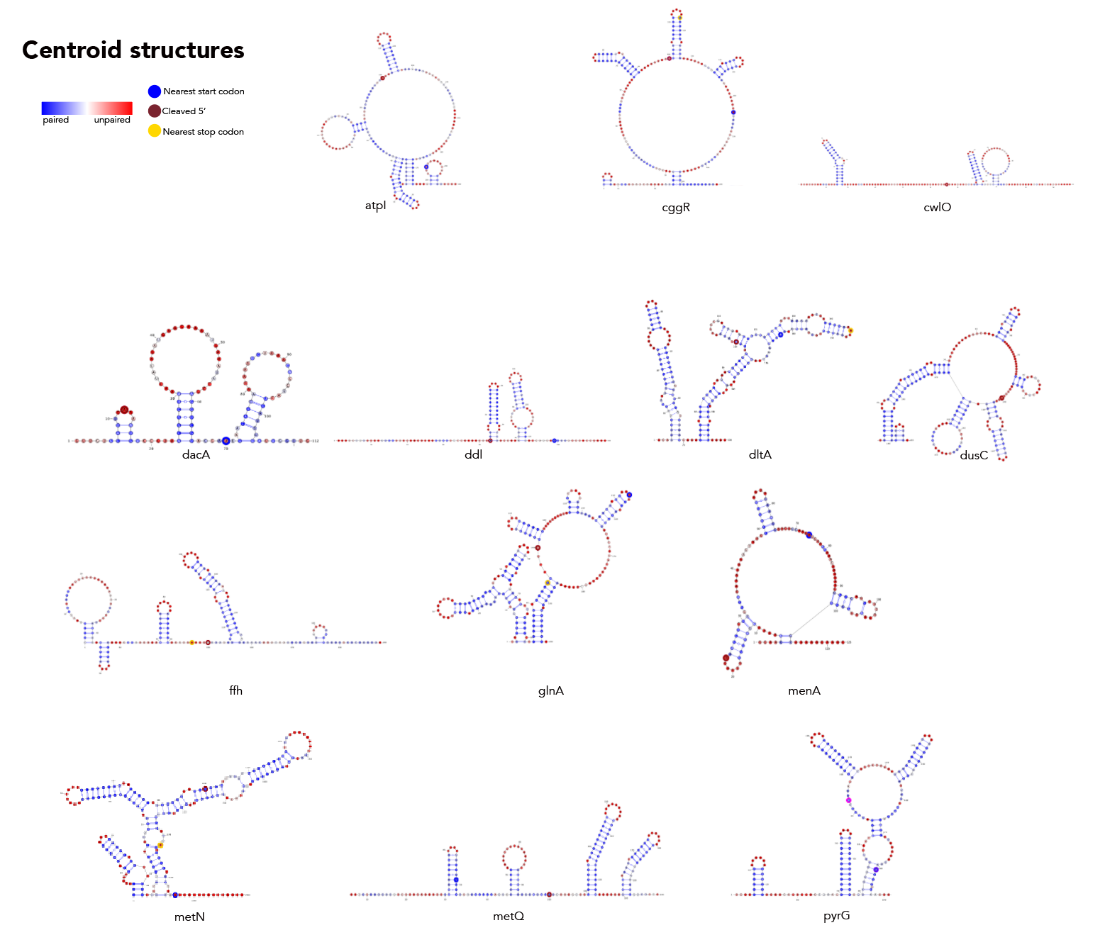
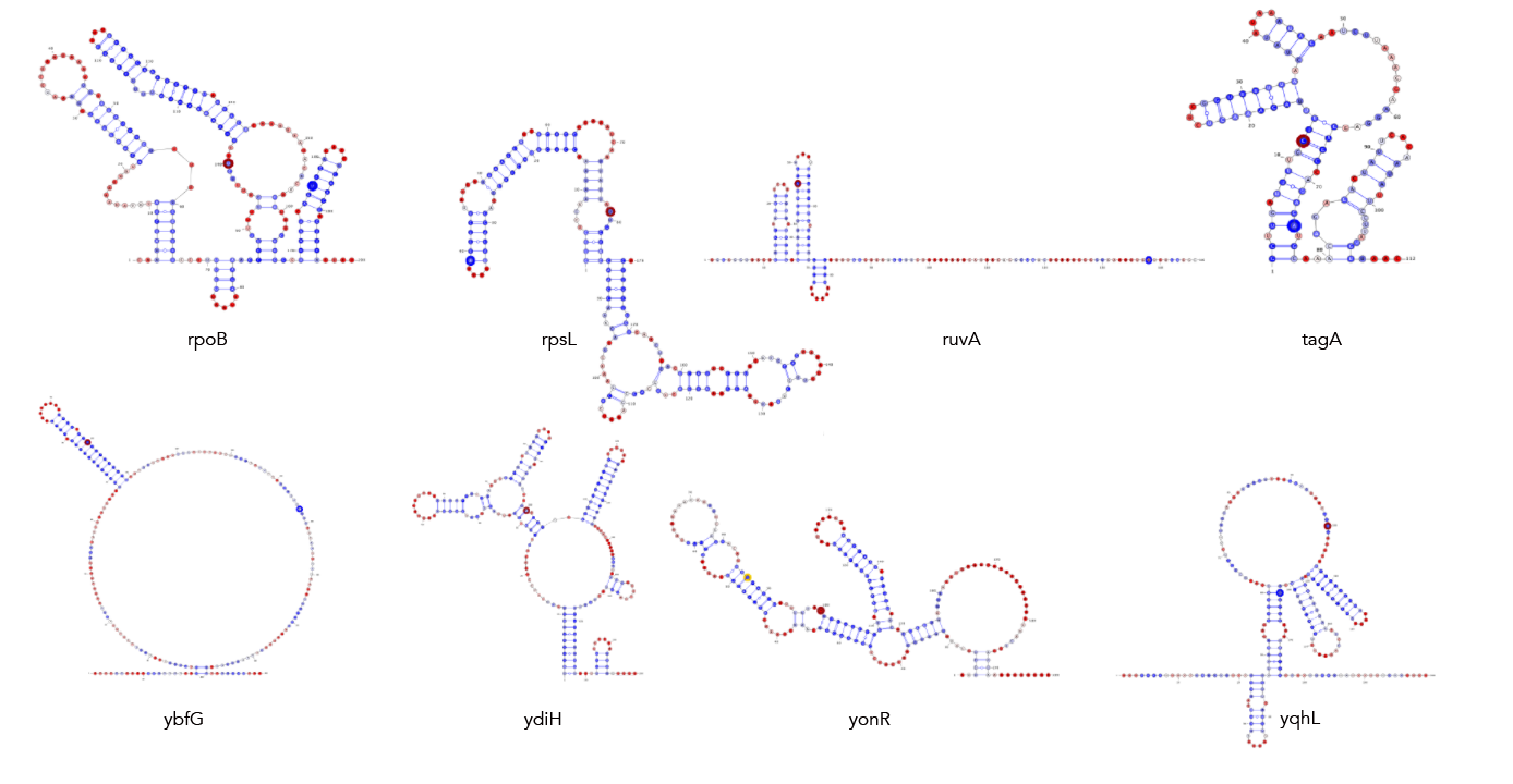
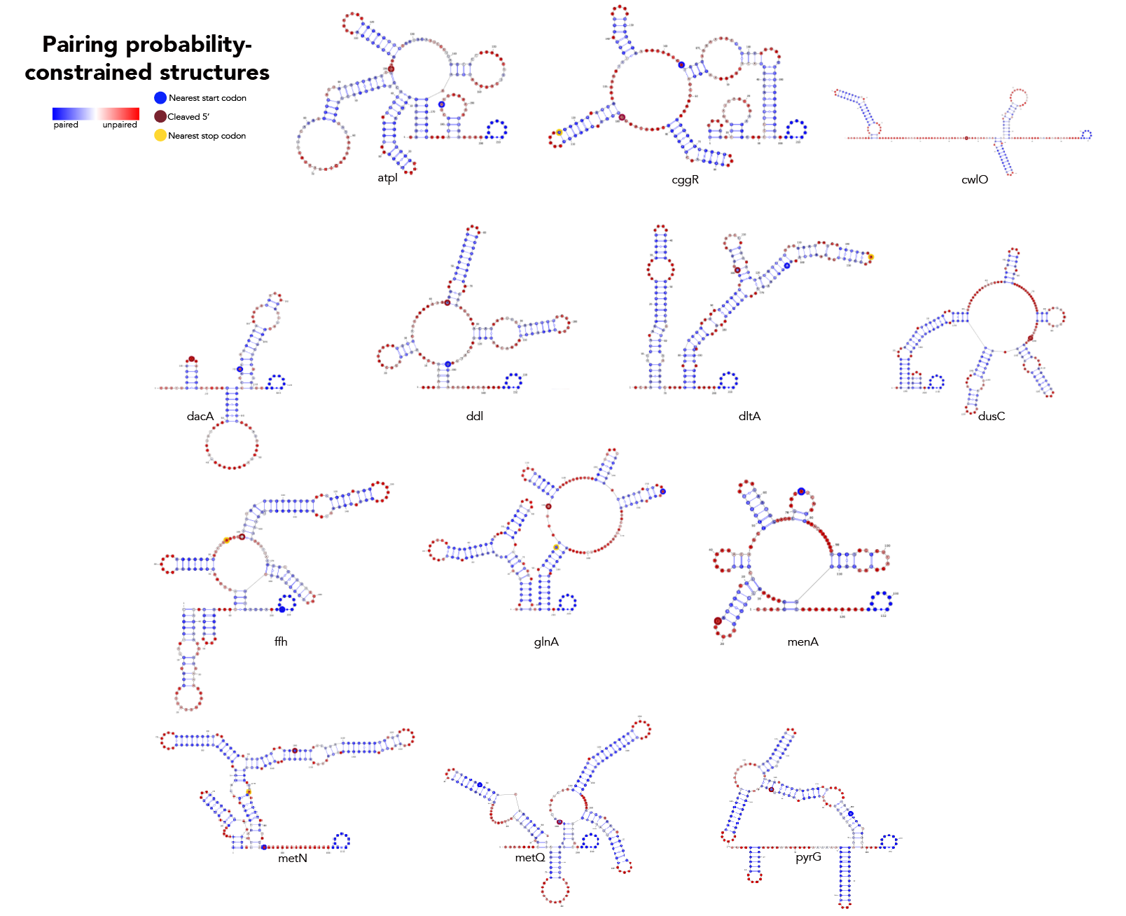
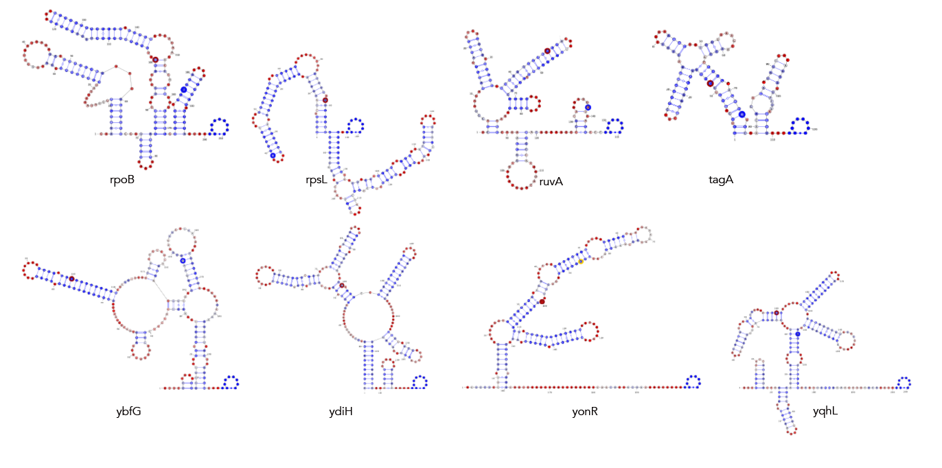
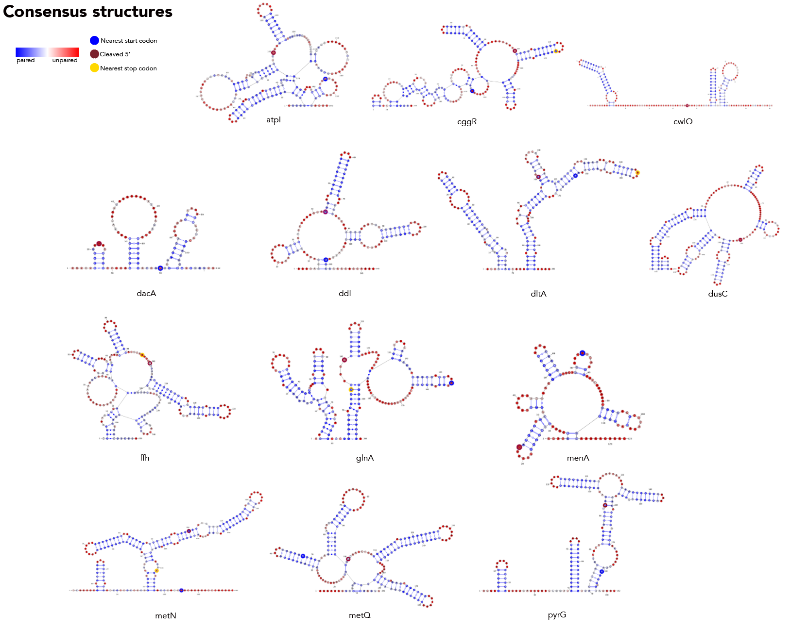
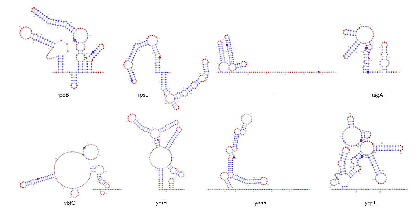
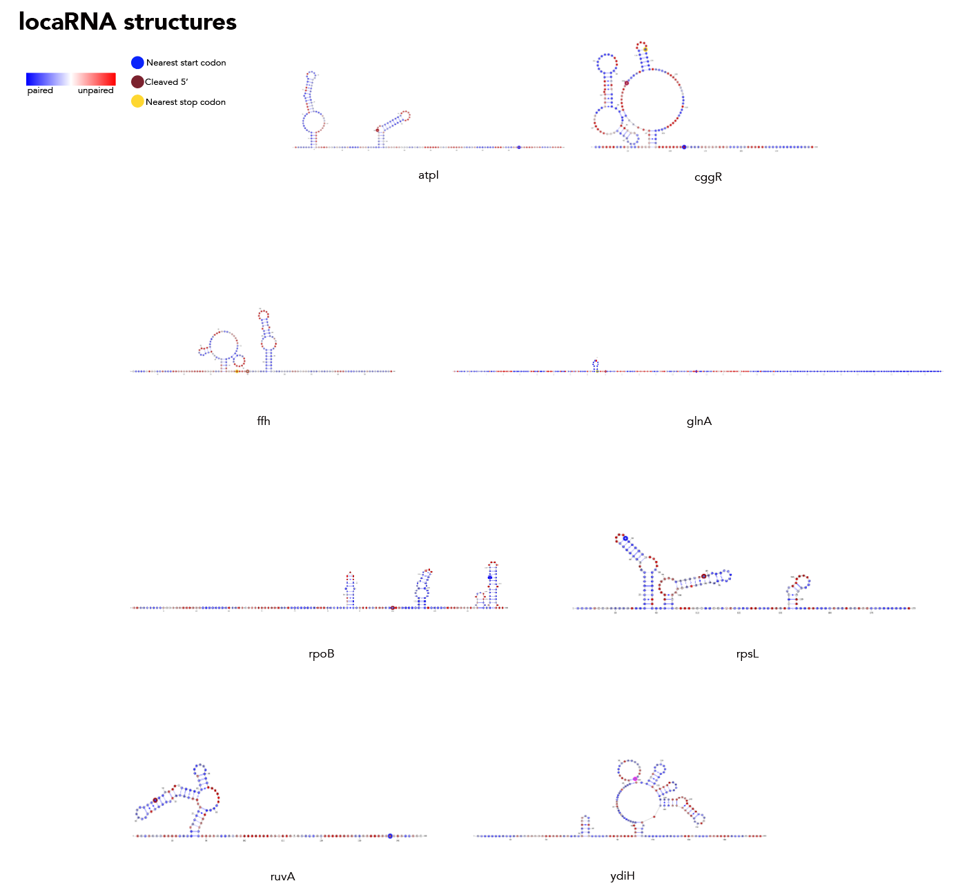
MFE, MEA, centroid and pairing probability-constrained structures are generated via RNAfold and visualized in VARNA. Consensus and locaRNA structures are also visualized in VARNA but generated separately.
If your RNAfold command isn't working, check that any "--" has actually translated properly to shell. Sometimes I found that -- was replaced with an emdash, which threw things off. More detailed descriptions for each fold below.
If you want to regenerate the structures, go to mfe/ and run rnafold --noPS --infile=21_cleavage_final.txt --outfile=21_cleavage_mfe.txt. From here, run mfe/separate_by_fasta_header.py to separate each structure into its own fasta-format file. You'll need to do this to visualize in varna. Otherwise you can just use *_mfe.txt under mfe/.
Then, you're going to want to run paired_prob/colormap_from_dat.py to get varna-compatible pairing probability colormaps for each site. Let's say you're interested in atpI--copy the numbers under "atpi reads:"
From here, go to mfe/ and run the following: java -cp path/to/VARNAv3-93.jar fr.orsay.lri.varna.applications.VARNAcmd -i atpi_mfe.txt -colorMapStyle "0.00:#0000FF,0.50:#FFFFFF,1.00:#FF0000" -colorMap [paste the colormap from colormap_from_dat here, leave a space between it and -colorMap].
If you want to regenerate the structures, go to mea/ and run rnafold --noPS --MEA --infile=21_cleavage_final.txt --outfile=21_cleavage_mea.txt. From here, run mea/separate_by_fasta_header.py to separate each structure into its own fasta-format file. Note that RNAfold prints out multiple structures given the MEA option. The first structure is the MFE and, unfortunately, if you pass a file with multiple structures to VARNA, it'll only print the first one. The last structure the --MEA option produces is the actual MEA structure. As such you'll need to delete any preceding structures to get a correct visualization.
Then, you're going to want to run paired_prob/colormap_from_dat.py to get varna-compatible pairing probability colormaps for each site. Let's say you're interested in atpI--copy the numbers under "atpi reads:"
From here, go to mea/ and run the following: java -cp path/to/VARNAv3-93.jar fr.orsay.lri.varna.applications.VARNAcmd -i atpi_mea.txt -colorMapStyle "0.00:#0000FF,0.50:#FFFFFF,1.00:#FF0000" -colorMap [paste the colormap from colormap_from_dat here, leave a space between it and -colorMap].
If you want to regenerate the structures, go to centroid/ and run rnafold --noPS -p --infile=21_cleavage_final.txt --outfile=21_cleavage_centroid.txt. From here, run mea/separate_by_fasta_header.py to separate each structure into its own fasta-format file. Note that RNAfold prints out multiple structures given the centroid option. The first structure is the MFE and, unfortunately, if you pass a file with multiple structures to VARNA, it'll only print the first one. The last structure the -p option produces is the actual centroid structure. As such you'll need to delete any preceding structures to get a correct visualization. Additionally, you need to get rid of the expression in curly braces after the structure. For some reason not doing so makes VARNA crash.
Then, you're going to want to run paired_prob/colormap_from_dat.py to get varna-compatible pairing probability colormaps for each site. Let's say you're interested in atpI--copy the numbers under "atpi reads:"
From here, go to centroid/ and run the following: java -cp path/to/VARNAv3-93.jar fr.orsay.lri.varna.applications.VARNAcmd -i atpi_centroid.txt -colorMapStyle "0.00:#0000FF,0.50:#FFFFFF,1.00:#FF0000" -colorMap [paste the colormap from colormap_from_dat here, leave a space between it and -colorMap].
This is a bit more complicated.
- paired_prob/separate_by_fasta_header.py on 21_cleavage_final.txt
- [again using atpI as the example] feed atpi.txt into paired_prob/produce_constraints.py to produce atpi_correct_constrained.txt
- in paired_prob run rnafold --noPS -p0 -C --infile=atpi_constrained.txt --outfile=atpi_constrained_structures.txt to get the constrained kTln(Z) values
- in paired_prob run rnafold --noPS -p0 --infile=atpi.txt --outfile=atpi_partition.txt to get the kTln(Z) value for the unconstrained structure
- feed "atpi" into paired_prob/boltzmann.py in the "name" field and run. This give you the .dat file atpi_paired_probs.dat.
- in paired_prob run rnafold --noPS --shape=atpi_paired_probs.dat --infile=atpi.txt --outfile=atpi_paired.txt
Then, you're going to want to run paired_prob/colormap_from_dat.py to get varna-compatible pairing probability colormaps for each site. Let's say you're interested in atpI--copy the numbers under "atpi reads:"
From here, stay in paired_prob and run the following: java -cp path/to/VARNAv3-93.jar fr.orsay.lri.varna.applications.VARNAcmd -i atpi_paired.txt -colorMapStyle "0.00:#0000FF,0.50:#FFFFFF,1.00:#FF0000" -colorMap [paste the colormap from colormap_from_dat here, leave a space between it and -colorMap].
Create the file consensus/atpi_structures.txt. Comments in the file must start with a # --these lines will be ignored. Separate each structure with a new line--e.g. #MFE \n [mfe structure]\n #MEA \n [mea structure]. Each *_structures.txt file must contain a MFE, MEA, centroid and pairing probability-constrained structure in no order. Just keep the dot-bracket structures, don't add anything else in. You don't need to add sequences to this file.
Use atpi_structures as input into consensus/consensus.py in addition to consensus/rna_atpi.txt--this outputs atpi_consensus.txt. You need the rna version because, while RNAfold will automatically convert T->U when generating a structure from a given sequence, the consensus approach does not. We don't want T's in varna structures so you need to take this step.
Then, you're going to want to run paired_prob/colormap_from_dat.py to get varna-compatible pairing probability colormaps for each site. Let's say you're interested in atpI--copy the numbers under "atpi reads:"
From here, move to consensus/ and run the following: java -cp path/to/VARNAv3-93.jar fr.orsay.lri.varna.applications.VARNAcmd -i atpi_consensus.txt -colorMapStyle "0.00:#0000FF,0.50:#FFFFFF,1.00:#FF0000" -colorMap [paste the colormap from colormap_from_dat here, leave a space between it and -colorMap].
Feed 21_cleavage_final.txt into locaRNA. From here copy the resulting consensus structure along with the subtilis sequence into a text file in locarna/. It's important that you copy the sequence and structure exactly as presented, dashes and all! From here input that sequence and structure into locarna/consensus_seq_structure.py to remove the dashes and get the consensus structure elements that correspond to the subtilis sequence.
Then, you're going to want to run paired_prob/colormap_from_dat.py to get varna-compatible pairing probability colormaps for each site. Let's say you're interested in atpI--copy the numbers under "atpi reads:"
From here, go to locarna/ and run the following: java -cp path/to/VARNAv3-93.jar fr.orsay.lri.varna.applications.VARNAcmd -i atpi_locarna.txt -colorMapStyle "0.00:#0000FF,0.50:#FFFFFF,1.00:#FF0000" -colorMap [paste the colormap from colormap_from_dat here, leave a space between it and -colorMap].
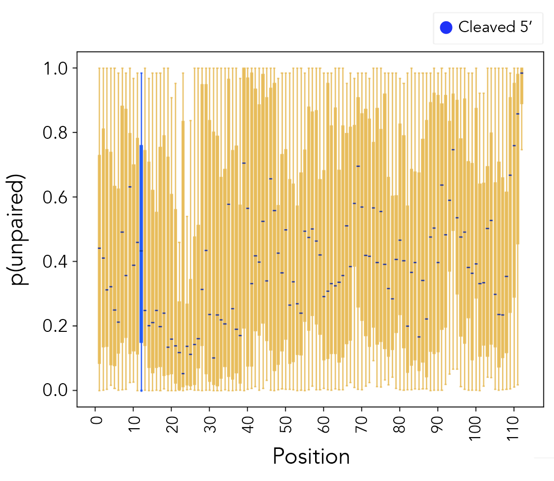
Run paired_prob/paired_prob_analysis.py.
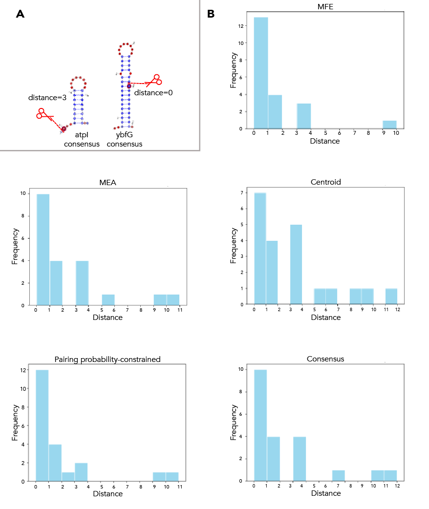
For all folds [MFE, MEA, centroid, pairing probability-constrained, consensus], navigate to their respective directories and run nearest_hairpin.py. You can also do this for locaRNA but doing so isn't particularly informative.
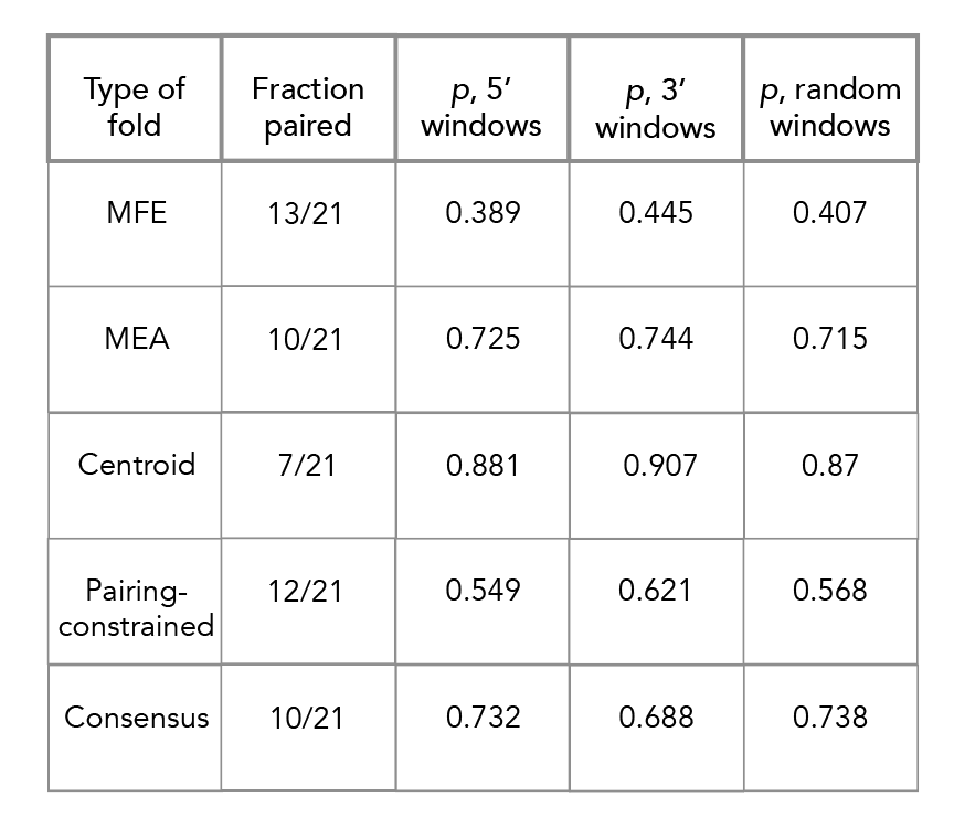
Navigate to p_value_analysis/. Each subdirectory corresponds to a different fold [locaRNA not included]. In each directory run select_21.py--this will produce the requisite p values. Change the input file names [*_3prime.txt, *_5prime.txt or *_random.txt] to determine p values for each background set. These scripts may take some time. Additional details available upon request.
