gblidar aims to make accessing LiDAR data from across Great Britain as easy as possible. It provides functions to search the Environment Agency’s LiDAR catalogue, download composite products, and merge the data into a single raster. It also provides functions to access the data from the EA’s WCS services, which is significantly faster but only available for some composite products. This package is still in development and only supports English data for now but will be expanded to include Scotland and Wales in the future.
- Added options for merging rasters and exporting as SpatRaster, stars of character.
- Generic merge for all rasters in gbl_catalog.
- Add special functions for hitting the WCS data to get faster access to large composite areas.
- Add Scottish Data
- Add Welsh Data
- Write Tests
You can install the development version of gblidar from GitHub with:
# install.packages("pak")
pak::pkg_install("h-a-graham/gblidar")This is a super quick demo where we can query the Environment Agency’s
entire LIDAR catalogue using the eng_search function. This will return
a gbl_catalog object which can be used to filter the assets and then
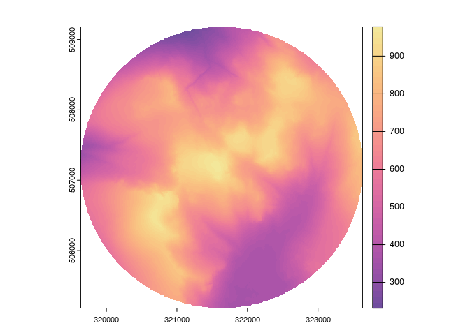
merge them into a single raster. In this example we search the area
around Scafell Pike, use the filter_catalog function to reduce the
number of assets to just the 2m DTM composite for 2022, and then use the
merge_assets function to merge all the assets into a single raster. By
default the raster is saved to disk and the
file path is returned, but this can be changed using raster_class
argument in merge_assets to return a stars or SpatRaster object
(or you can alternatively set the global option
gblidar.out_raster_type to “stars” or “SpatRaster” as in the example
below).
library(gblidar)
library(sf)
#> Linking to GEOS 3.12.1, GDAL 3.8.3, PROJ 9.3.1; sf_use_s2() is TRUE
if (rlang::is_installed("terra")) {
  library(terra)
  options(gblidar.out_raster_type = "SpatRaster")
}
#> terra 1.7.71

scafell_box <- st_point(c(321633, 507181)) |>
  st_buffer(2000) |>
  st_sfc() |>
  st_set_crs(27700)

scafell_catalog <- eng_search(scafell_box)

print(scafell_catalog)
#> Data Catalog
#> # A tibble: 28 × 5
#>    product                                   resolution  year filenames urls
#>    <chr>                                          <dbl> <int> <list>    <list>
#>  1 LIDAR Composite DTM                                1  2022 <chr [9]> <chr>
#>  2 LIDAR Composite DTM                                2  2022 <chr [9]> <chr>
#>  3 LIDAR Composite First Return DSM                   1  2022 <chr [9]> <chr>
#>  4 LIDAR Composite First Return DSM                   2  2022 <chr [9]> <chr>
#>  5 LIDAR Composite Last Return DSM                    1  2022 <chr [9]> <chr>
#>  6 LIDAR Composite Last Return DSM                    2  2022 <chr [9]> <chr>
#>  7 LIDAR Point Cloud                                 NA  2008 <chr [1]> <chr>
#>  8 LIDAR Point Cloud                                 NA  2009 <chr [8]> <chr>
#>  9 LIDAR Tiles DSM                                    1  2007 <chr [2]> <chr>
#> 10 LIDAR Tiles DSM                                    1  2008 <chr [3]> <chr>
#> 11 LIDAR Tiles DSM                                    1  2009 <chr [8]> <chr>
#> 12 LIDAR Tiles DSM                                    2  2000 <chr [2]> <chr>
#> 13 LIDAR Tiles DTM                                    1  2007 <chr [2]> <chr>
#> 14 LIDAR Tiles DTM                                    1  2008 <chr [3]> <chr>
#> 15 LIDAR Tiles DTM                                    1  2009 <chr [8]> <chr>
#> 16 LIDAR Tiles DTM                                    2  2000 <chr [2]> <chr>
#> 17 National LIDAR Programme DSM                       1  2019 <chr [7]> <chr>
#> 18 National LIDAR Programme DSM                       1  2021 <chr [2]> <chr>
#> 19 National LIDAR Programme DTM                       1  2019 <chr [7]> <chr>
#> 20 National LIDAR Programme DTM                       1  2021 <chr [2]> <chr>
#> 21 National LIDAR Programme First Return DSM          1  2019 <chr [7]> <chr>
#> 22 National LIDAR Programme First Return DSM          1  2021 <chr [2]> <chr>
#> 23 National LIDAR Programme Intensity                 1  2019 <chr [7]> <chr>
#> 24 National LIDAR Programme Intensity                 1  2021 <chr [2]> <chr>
#> 25 National LIDAR Programme Point Cloud               1  2019 <chr [7]> <chr>
#> 26 National LIDAR Programme Point Cloud               1  2021 <chr [2]> <chr>
#> 27 National LIDAR Programme VOM                       1  2019 <chr [7]> <chr>
#> 28 National LIDAR Programme VOM                       1  2021 <chr [2]> <chr>
#> AOI Geometry
#> Geometry set for 1 feature
#> Geometry type: POLYGON
#> Dimension:     XY
#> Bounding box:  xmin: 319633 ymin: 505181 xmax: 323633 ymax: 509181
#> Projected CRS: OSGB36 / British National Grid
#> POLYGON ((323633 507181, 323630.3 507076.3, 323...
#> Tile Names
#> [1] "NY10NE" "NY20NW"

DTM_catalog <- scafell_catalog |>
  filter_catalog(
    product == "LIDAR Composite DTM",
    resolution == 2,
    year == 2022
  )

print(DTM_catalog)
#> Data Catalog
#> # A tibble: 1 × 5
#>   product             resolution  year filenames urls
#>   <chr>                    <dbl> <int> <list>    <list>
#> 1 LIDAR Composite DTM          2  2022 <chr [9]> <chr [9]>
#> AOI Geometry
#> Geometry set for 1 feature
#> Geometry type: POLYGON
#> Dimension:     XY
#> Bounding box:  xmin: 319633 ymin: 505181 xmax: 323633 ymax: 509181
#> Projected CRS: OSGB36 / British National Grid
#> POLYGON ((323633 507181, 323630.3 507076.3, 323...
#> Tile Names
#> [1] "NY10NE" "NY20NW"

scafell_raster <- merge_assets(DTM_catalog, mask = TRUE)

plot(scafell_raster, col = grDevices::hcl.colors(50, palette = "Sunset"))
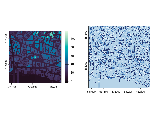
The EA have now released their latest composite products as WCS services
(Awesome!). To make best use of this, we provide the eng_composite
function which can be used to directly download only the data you need
for any area in England. This is significantly faster than the
eng_search function and is preferred if you are only interested in the
latest composite products. Both elevation and hillshade data are
available for “fz_dsm” (first return DSM), “dsm”, “dtm”, and “vom”.
options(gblidar.progress = FALSE) # for readability in this example.

search_box <- st_point(c(532054, 181145)) |>
  st_buffer(500) |>
  st_sfc() |>
  st_set_crs(27700)

# the elevation data for the first return DSM
fz_dsm <- eng_composite(search_box, product = "fz_dsm")
# the hillshade data for the last return DSM
dsm_hs <- eng_composite(search_box, product = "dsm", product_type = "hillshade")

par(mfrow = c(1, 2))
plot(fz_dsm, col = hcl.colors(150, "mako"))
plot(dsm_hs, col = hcl.colors(256, "Blues"), legend = FALSE)

