This repository is a companion to a lecture given at the University of Cambridge Engineering Department, which is available for viewing here. In it you will find the code to reproduce all of the visualizations and experiments shared in the lecture, as well as a Jupyter Notebook providing interactive lecture notes convering the following topics:
- 1D Signal Reconstruction
- 2D Image Regression
- Volume Raycasting
- 3D Volume Rendering with NeRF
In this section I will outline how to run the various experiments. Before I begin, it is worth noting that while the defaults are all reasonable and will produce the results you see in the lecture, it can be very educational to play around with different hyperparameter values and observe the results.
In order to run the various experiments, you will first need to install the requirements for the repository, ideally in a virtual environment. We recommend using a version of Python >= 3.7. As this code heavily relies upon PyTorch, you should install the correct version for your platform. The guide here is very useful and I suggest you follow it closely. You may also find this site helpful if you are working on Windows. Once that is done, you can run the following:
pip install wheel
pip install -r requirements.txt
You should now be ready to run any of the experiment scripts in this repository.
This repository contains implementations of the research presented in Fourier Features Let Networks Learn High Frequency Functions in Low Dimensional Domains and NeRF: Representing Scenes as Neural Radiance Fields for View Synthesis. Those who use this code should be sure to cite them, and to also take a look at our own work in this space, FastNeRF: High-Fidelity Neural Rendering at 200FPS.
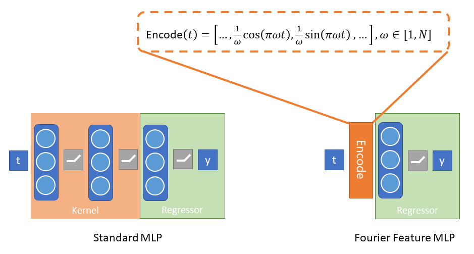
Fourier Feature Networks address the inherent problems with teaching neural nets to model complex signals from low frequency information. They do this by introducing Fourier features as a preprocessing step, used to encode the low-frequency inputs in such a way as to introduce higher-frequency information as seen below for the 1D case:
Ultimately the Fourier features replace the featurizer, or kernel, that the neural net would otherwise need to learn. As shown above, Fourier Feature Networks can be used to predict a 1-D signal from a single floating point value indicating time. They can also be used to predict image pixel values from their position and, most intriguingly, predict color and opacity from 3D position and view direction, i.e. to model a radiance field. The ability to do that allows the creation of rendered neural avatars, like the one below:
neural_rendered_avatar.mp4
As well as neurally rendered objects which have believable materials properties and view-dependent effects.
The code contained in this repository is intended for use as supplemental learning materials to the lecture. The Lecture Notes in particular will provide a walkthrough of the technical content. This README is focused more on how to run these scripts to reproduce experimental results and/or run your own experiments using this code.
As in the lecture, you can access any of a variety of datasets for use in running these (or your own) experiments:
The SignalDataset class can take any function
mapping a single input to a single output. Feel free to experiment.
Here is an example of how to create one:
def _multifreq(x):
    return np.sin(x) + 0.5*np.sin(2*x) - 0.2*np.cos(5*x) + 2

num_samples = 32
sample_rate = 8
dataset = ffn.SignalDataset.create(_multifreq, num_samples, sample_rate)The PixelDataset class can take any path to an
image. Create one like this:
dataset = ffn.PixelDataset.create(path_to_image_file, color_space="RGB",
size=512)This is where the library becomes a bit picky about input data. The
ImageDataset supports a set format for data,
and we provide several datasets in this format to play
with. These datasets are not stored in the repo, but the library will
automatically download them to the data folder when you first requests them
which you can do like so:
dataset = ffn.ImageDataset.load("antinous_400.npz", split="train", num_samples=64)We recommend you use one of the following (all datasets are provided in 400 and 800 versions):
| Name | Image Size | # Train | # Val | # Test | Description | Sample image |
|---|---|---|---|---|---|---|
antinous_(size) |
(size)x(size) | 100 | 7 | 13 | Renders of a sculpture kindly provided by the Fitzwilliam Museum. Does not include view-dependent effects. | 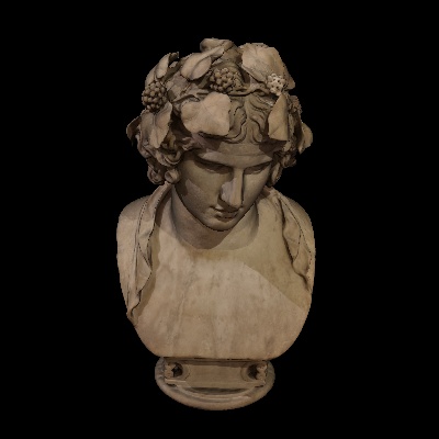 |
rubik_(size) |
(size)x(size) | 100 | 7 | 13 | This work is based on "Rubik's Cube" (https://sketchfab.com/3d-models/rubiks-cube-d7d8aa83720246c782bca30dbadebb98) by BeyondDigital (https://sketchfab.com/BeyondDigital) licensed under CC-BY-4.0 (http://creativecommons.org/licenses/by/4.0/). Does not include view-dependent effects. | 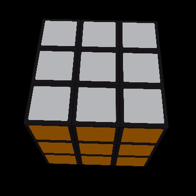 |
lego_(size) |
(size)x(size) | 100 | 7 | 13 | Physically based renders of a lego build, provided by the NeRF authors. | 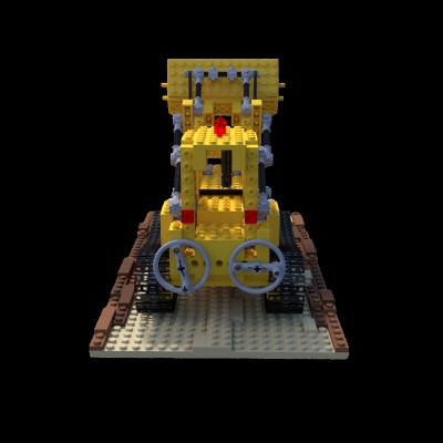 |
trex_(size) |
(size)x(size) | 100 | 7 | 13 | This work is based on "The revenge of the traditional toys" (https://sketchfab.com/3d-models/the-revenge-of-the-traditional-toys-d2dd1ee7948343308cd732c665ef1337) by Bastien Genbrugge (https://sketchfab.com/bastienBGR) licensed under CC-BY-4.0 (http://creativecommons.org/licenses/by/4.0/). Rendered with PBR and thus includes multiple view-dependent effects. | 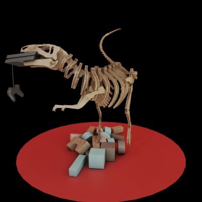 |
benin_(size) |
(size)x(1.5 *size) | 74 | 10 | 0 | Free moving, hand-held photographs of a bronze statue of a rooster from Benin, kindly provided by Jesus College, Cambridge. | 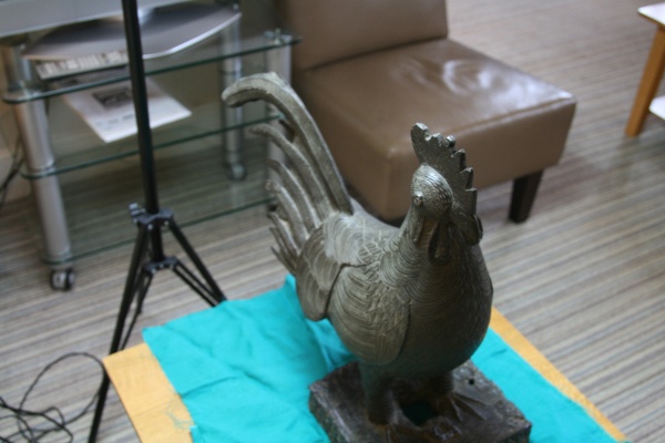 |
matthew_(size) |
(size)x(size) | 26 | 5 | 0 | Photographs of me, taken by a 31 camera fixed rig. | 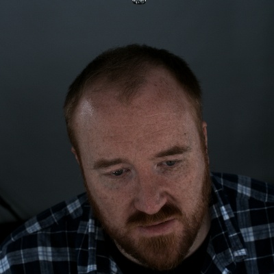 |
If you want to bring your own data, the format we support is an NPZ with the following tensors:
| Name | Shape | dtype | description |
|---|---|---|---|
| images | (C, D, D, 4) | uint8 | Tensor of camera images with RGBA pixel values. Alpha value indicates a mask around the object (where appropriate). |
| intrinsics | (C, 3, 3) | float32 | Tensor of camera intrinsics (i.e. projection) matrices |
| extrinsics | (C, 4, 4) | float32 | Tensor of camera extrinsics (i.e. camera to world) matrices |
| bounds | (4, 4) | float32 | Rigid transform indicating the bounds of the volume to be rendered. Will be used to transform a unit cube. |
| split_counts | (3) | int32 | Number of cameras (in order) for train, val and test data splits. |
where C is the number of cameras and D is the image resolution. You may find
it helpful to use the provided datasets as a reference.
These experiments form the basis of the results that you may have already seen in the lecture. With a sufficiently powerful GPU (or access to one in Azure or another cloud service) you should be able to reproduce all the animations and videos you have seen. In this section, I will provide a brief guide to how to use the different scripts that you will find in the root directory of the repo.
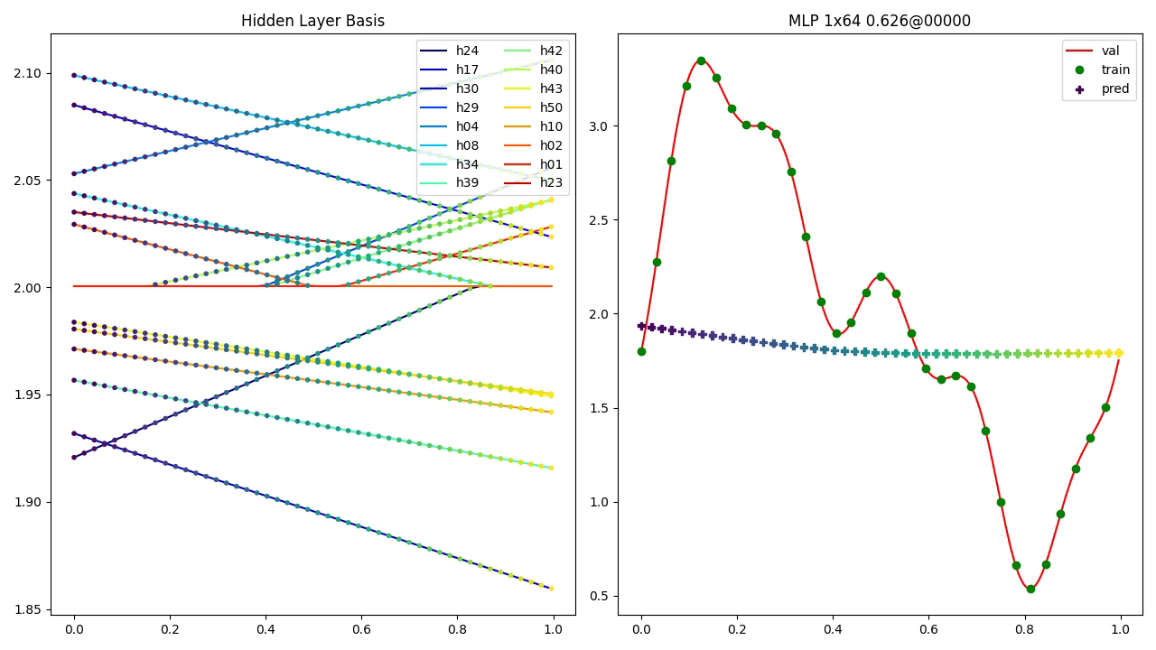
The 1D Signal Regression script can be invoked like so:
python train_signal_regression.py multifreq outputs/multifreq
You should see a window pop up that looks like the image below:
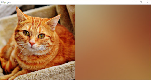
To get started with 2D Image Regression, run the following command:
python train_image_regression.py cat.jpg mlp outputs/cat_mlp
A window should pop up as the system trains that looks like this:
At the end it will show you the result, which as you will have come to
expect from the lecture is severaly lacking in detail due to the lack
of high-frequency gradients. Try running the same script with
positional or gaussian in place of mlp to see how using
Fourier features dramatically improves the quality. Your results should
look like what you see below:
ir_pos.mp4
Feel free to pass the script your own images and see what happens!
As a preparation for working with volume rendering, it can be useful to get a feel for the training data. If you run:
python test_ray_sampling.py lego_400.npz lego_400_rays.html
This should download the dataset into the data directory and then create
a scenepic showing what the ray sampling data looks like. Notice how the rays
pass from the camera through the pixels and into the volume. Try running
this script again with --stratified to see what happens when we add some
uniform noise to the samples. Here is an example of what this can look like:
ray_sampling_crop.mp4
Just like in the lecture, we'll start with voxel-based rendering. If you run the following command:
python train_voxels.py lego_400.npz 128 outputs/lego_400_vox128
You should be able to train a voxel representation of a radiance field.
Note You may have trouble running this script (and the ones that follow) if your computer does not have a GPU with enough memory. See Running on Azure ML for information on how to run these experiments in the cloud.
If you look in the train and val folders in the output
directory you can see images produced during training showing how
the model improves over time. There is also a visualization of the
model provided in the voxels.html scenepic. Here is an example
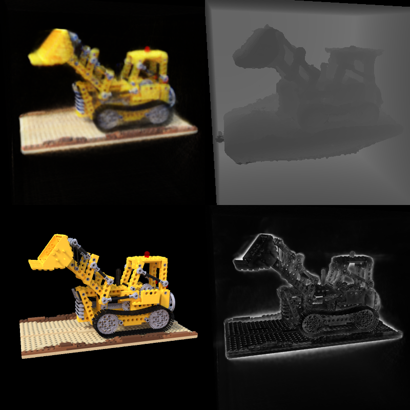
of an image produced by the Ray Caster:
All of the 3D methods will produce these images when in default training mode. They show (in row major order): rendered image, depth, training/val image, and per-pixel error. You can also ask the script to make a video of the training process. For example, if you run this script:
python train_voxels.py lego_400.npz 128 outputs/lego_400_vox128 --make-video
It will produce the frames of the following video:
lego_400_vox128_train.mp4
Another way to visualize what the model has learned is to produce a voxelization of the model. This is different from the voxel-based volume rendering, in which multiple voxels contribute to a single sample. Rather, it is a sparse octree containing voxels at the places the model has determined are solid, thus providing a rough sense of how the model is producing the rendered images. You can produce a scenepic showing this via the following command:
python voxelize_model.py outputs/lego_400_vox128/voxels.pt lego_400.npz lego_400_voxels.html
This will work for any of the volumetric rendering models.
The first neural rendering technique we looked at was so-called "Tiny" NeRF, in which the view direction is not incorporated but we only focus on the 3D position within the volume. You can train Tiny NeRF models using the following command:
python train_tiny_nerf.py lego_400.npz mlp outputs/lego_400_mlp/
Substituting positional and gaussian as before to try out different modes
of Fourier encoding. You'll notice again the same low-resolution results for
MLP and similarly improved results when Fourier features are introduced. Here
is a side-by-side comparison of mlp and positional training for our
datasets (top row is nearest training image to the orbit camera).
Your results should be similar.
tiny_nerf_pos.mp4
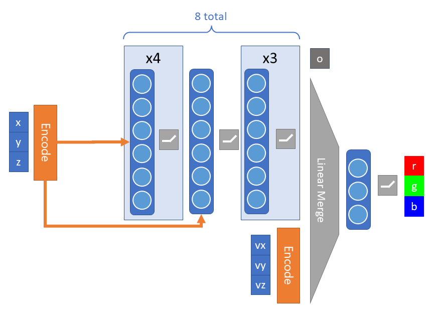
In the results above you possibly noticed that specularities and transparency were not quite right. This is because those effects require the incorporation of the view direction, that is, where the camera is located in relation to the position. NeRF introduces this via a novel structure in the fairly simple model we've used so far:
First, the model is deeper, allowing it to encode more information about the radiance field (note the skip connection to address signal attenuation with depth). However, the key structure difference is the addition of the ray direction being added before the final layer. A subtle but important point is that the opacity is predicted without the view direction, to encourage structural consistency.
The other major difference from what has come before is that NeRF samples
the volume in a different way. The technique performs two-tiers of sampling.
First, they sample a coarse network, which determines where in the space
is opaque, and then they use that to create a second set of samples which
are used to train a fine network. For the purpose of this lecture, we do
something very similar in spirit, which is to use the voxel model we trained
above as the coarse model. You can see how this changes the sampling of the
volume by running the test_ray_sampling.py script again:
python test_ray_sampling.py lego_400.npz lego_400_fine.html --opacity-model lego_400_vox128.pt
You should now be able to see how additional samples are clustering near
the location of the model, as opposed to being only evenly distributed over
the volume. This helps the NeRF model to learn detail. Try passing in
--stratified again to see the effects for random sampling as well. The video
below displays the results of different kinds of sampling, but you should
explore it for yourself as well:
sampling.mp4
Note The Tiny NeRF model can also take advantage of fine sampling using an opacity model. Try it out!
You can train the NeRF model with the following command:
python train_nerf.py lego_400.npz outputs/lego_400_nerf --opacity-model lego_400_vox128.pt
While this model can train for many more steps than 50000 and continue to improve, you should already be able to see the increase in quality over the other models from adding in view direction. Here are some sample render orbits from the NeRF model:
antinous_800_nerf.mp4
lego_800_nerf.mp4
trex_800_nerf.mp4
You can produce these orbit videos yourself by calling, for example:
python orbit_video.py antinous_800_nerf.pt 800 outputs/antinous_render --opacity-model antinous_800_vox128.pt
Give it a try! That's it for the main experimental scripts. All of them have descriptive help statements, so be sure to explore your options and see what you can learn.
It is outside of the scope of this lecture (or repository) to describe in detail
how to get access to cloud computing resources for machine learning via
Azure ML. However, there are some amazing resources out there already.
For the purpose of this repository, all you need to do is complete
this Quickstart Tutorial
and download the config.json associated with your workspace into the root
of the repository. You can then run any of the training scripts in Azure ML
using the submit_aml_run.py script, like so:
python submit_aml_run.py cat <compute> train_image_regression.py "cat.jpg mlp outputs"
Where cat is the experiment name (you can choose anything here) that will
group different runs together, and where you replace <compute> with the
name of the compute target you want to use to run the experiment (which
will need to have a GPU available). Finally you provide the script name
(in this case, train_image_regression.py, which I suggest you use while you
are getting your workspace up and running) and the arguments to the script as
a string. If you get an error, make certain you've run:
pip install -r requirements-azureml.txt
If everything is working, you should receive a link that lets you monitor the experiment and view the output images and results in your browser.
