sphstat: A Python 3 package for spherical statistics

Description

Spherical data arises in many different fields of science. sphstat (pronouced siff-stæt) provides the necessary tools to apply inferential statistics on data on the unit sphere. The package implements tests and algorithms for vectorial datagiven by Fisher, Lewis and Embleton [1]. Note that tests and methods for axial data have not yet been implemented as of version 1.0

Author

Huseyin Hacihabiboglu, METU Spatial Audio Research Group (SPARG), Ankara, Turkiye
Github: @hacihabiboglu
E-mail: hhuseyin@metu.edu.tr

Installation

Option 1

sphstat can be installed from PyPI using pip3. In Terminal, type

  pip3 install sphstat

Option 2

Alternatively you can download it from Github as a ZIP file or as a Git repository:

git clone https://github.com/metu-sparg/sphstat
cd PATH/TO/LOCAL/FOLDER
pip3 install .

Documentation is available at https://sphstat.readthedocs.io/en/latest/

Requirements

sphstat was tested on an Apple M1 computer with Python 3.10. It is agnostic of the platform and will very likely work on Python 3.8 and above.

numpy
scipy
sympy
openpyxl
pandas
matplotlib

Usage and examples

sphstat implements includes several modules whose names are pretty self-explanatory. These are:

descriptives: Functions for descriptive statistics on spherical data
distributions: Functions for generating data from different spherical distributions
singlesample: Functions for single-sample tests on spherical data
twosample: Functions for inferential staticts on two or more samples
modelling: Functions for cross-correlation, regression, and temporal analysis
utils: Utility functions used by other modules

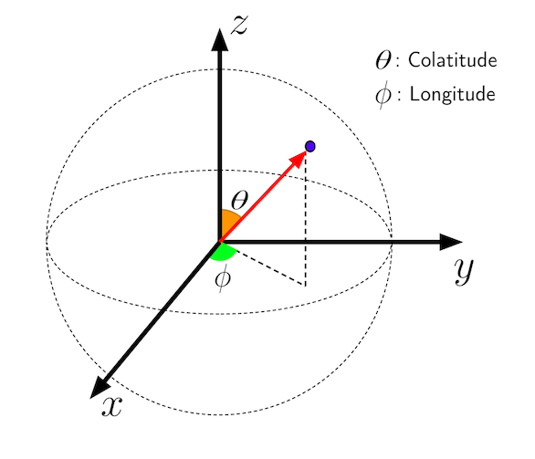
It is important to note that the default coordinate system used by sphstat is the polar coordinates. The colatitude angle ($theta$) is defined from the axis, $0$ (north pole) to $\pi/2$ (south pole) and the latitude angle is defined from $0$ (front direction) to $2\pi$. Figure shows the employed polar coordinate system.

A full documentation is available at readthedocs.

The following examples demonstrate the usage of sphstat.

Importing `sphstat`

After installation, sphstat is imported just like any other Python package by:

import sphstat

Reading and converting a sample

Presently only Excel files are accepted as input. Each worksheet should contain a single sample. Data can either be in degrees or in radians. Data in three different spherical coordinate systems can be processed. The default system is polar, but longitude/latitute (i.e. 'lonlat') and declination/inclination (i.e. 'decinc') can also be handled. While some functions require data in polar coordinates, some others will require a Cartesian representation. Necessary conversions need to be made. The following example shows reading data in the second worksheet, represented in declination/inclination form (e.g. Dec. in first column and Inc. in the second) in radians and converted to first to polar coordinates and then to Cartesian form:

from utils import readsample, convert, polartocart
    
sample = readsample('/PATH/TO/DATA/mydata.xlsx', wsindex=1, typ='rad')
samplepol = convert(sample, 'decinc')
samplecart = polartocart(samplepol)

Descriptive statistics of spherical data

The descriptive statistics of spherical data is obtained by using the resultants() function from

from descriptives import resultants
from utils import prettyprintdict

r = resultants(samplecart)
prettyprintdict(r)

Directional Cosines:  [ 0.22649571 -0.07068299  0.97144408]
Resultant Vector:  [ 8.0846443  -2.52299178 34.67518128]
Resultant Length:  35.694469568249374
Mean Direction:  (0.23955319922943338, -0.30249497353817606)
Mean Resultant Length:  0.9915130435624826

Another useful function is mediandir() which calculated the median direction as well as the parameters for (1-alpha)% confidence cone:

from descriptives import mediandir

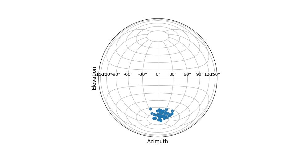
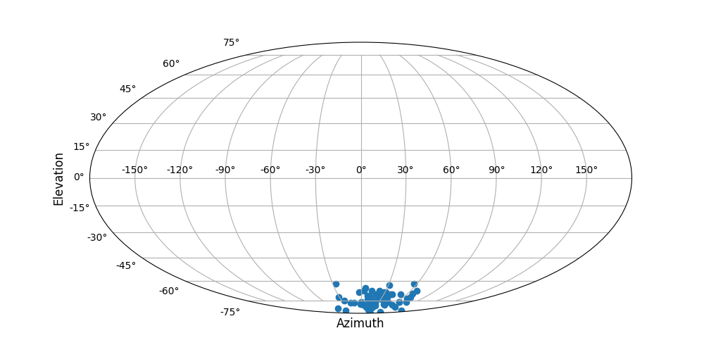
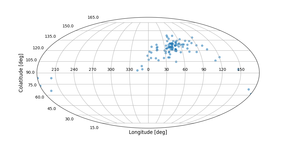
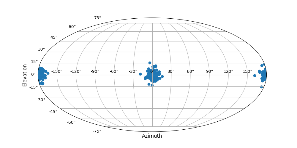
medi, ccone, success, W = mediandir(samplecart, ciflag=True, alpha=0.01)

Plotting a sample

sphstat uses either one of Mollweide or Lambert projections to display data.

from plotting import plotdata

plotdata(sample,  proj='lambert')
plotdata(sample,  proj='mollweide')

will produce the following scatterplots, respectively.

Lambert projection:

Mollweide projection:

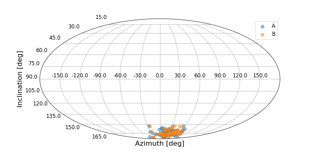
Multiple data plot

Two or more data can also be overlaid. plotdatalist() will produce the necessary legend for the scatterplot:

from plotting import plotdatalist

samplelist = [sampleA, sampleB]
plotdatalist(samplelist, labels=['A', 'B'], proj='mollweide')

Generating samples from spherical distributions

sphstat.distributions provides functions that can generate vectors randomly drawn from uniform, Fisher, Kent and Watson distributions

from sphstat.distributions import kent

mu0 = np.array([0., 1., 0.])
sample = kent(100, 50, 20, np.array([1., 1., 1.]), mu0)
samplerad = carttopolar(sample)
plotdata(samplerad, proj='mollweide')

samplewatson = watson(100, lamb=0., mu=1., nu=0., kappa=50)
samplerad = carttopolar(samplewatson)
splt.plotdata(samplerad, proj='mollweide')

Statistics on a single sample

sphstat.singlesample contains different tests and parameter estimators for a single sample. For example, testing whether a sample comes from a uniform distribution:

from sphstat.singlesample import isuniform

res = isuniform(samplecart, alpha=0.05)
prettyprintdict(res)

teststat:  86.04615038397233
crange:  7.814727903251179
testresult:  False

...or Fisher distribution (which provides the results of three different tests for Fisherianness):

from sphstat.singlesample import isfisher

res = isfisher(samplecart, alpha=0.05)
prettyprintdict(res)

colatitute:  {'stat': 0.9137353833832544, 'crange': 1.094, 'H0': True}
longitude:  {'stat': 1.5941243439349297, 'crange': 1.207, 'H0': False}
twovariable:  {'stat': 0.7669521350409133, 'crange': 0.895, 'H0': True}
H0:  False
alpha:  0.05

Parameter estimation functions output multiple values. For example, fisherparams() will output mean direction, concentration parameters, semi-vertical angle, and (1-alpha)% CI for the concentration parameter:

from sphstat.singlesample import fisherparams

mdir, kappa, thetaalpha, cikappa = fisherparams(samplecart, alpha=0.05)

There are also functions to test the sample statistics against hypothethical values. For example, whether the population concentration parameter is a given value can be tested:

from sphstat.singlesample import kappatest

res = kappatest(samplecart, kappa0 = 100)
prettyprintdict(res)

R:  30.765364522847698
cvaltup:  (32.781120236887155, 32.559979744967514)
testresult:  False

Statistics on two or more samples

The tests and methods in sphstat.twosample provides tests and methods for the analysis and comparison of multiple vectorial samples on the unit sphere. For example, in the following example, three samples are tested for a common mean direction.

from sphstat.twosample import iscommonmean
from sphstat.utils import polartocart, convert

sample1rad = convert(sample1, 'decinc')
sample2rad = convert(sample2, 'decinc')
sample3rad = convert(sample3, 'decinc')
slist = [sample1rad, sample2rad, sample3rad] #, sample3, sample4]
slistcart = []
for s in slist:
    slistcart.append(polartocart(s))

res = iscommonmean(slistcart, alpha=0.05)
prettyprintdict(res)

Gr:  9.543041349403211
cval:  9.487729036781154
testresult:  False

There are also more specific tests if, for example, it is known that the underlying distributions are Fisher, a multiple comparison akin to running multiple t-tests on linear data is given by

from sphstat.twosample import isfishercommonmean

res = isfishercommonmean(slistcart)
prettyprintdict(res)

Z:  0.9921425881206186
z0:  0.992171530518573
res:  True

Similarly, a test similar to Levene's test for testing whether multiple samples have the same concentration parameter is:

from sphstat.twosample import isfishercommonkappa

res = isfishercommonkappa(slistcart)
prettyprintditc(res)

Z:  4.853124235595307
cval:  5.991464547107979
df:  2
testresult:  True

Correlation, regression, temporal association

Functions in sphstat.modelling implement functionality to calculate correlations, regression and time-series analysis on spherical data. For example:

from sphstat.modelling import xcorrrandomsamples

res = xcorrrandomsamples(sampcart1, sampcart2, 10000, htype='!=', alpha=0.05)
prettyprintdict(res)

rhohat:  0.8512942745968715
std:  0.03355675208163771
cval:  (-0.0661660798549282, -0.12290819705298231)
ci:  (0.7855242490787221, 0.9170643001150208)
testresult:  True

indicates that two samples are correlated with a correlation coefficient of $0.851$ with the 95% confidence interval also given.

In order to check if there is any serial association between time-ordered observations in a sample:

from sphstat.modelling import isn

res = isnotseriallyassociated(sampcart, alpha=0.05)
prettyprintdict(res)

Sstar:  2.504563022268227
cval:  1.6448536269514722
testresult:  False

indicating that the observations are not serially associated at $\alpha=0.05$ level.

Limitations

In its present version sphstat...

...mostly works on larger (i.e. n >= 25) sample sizes. While some bootstrapped methods (e.g. jackknife and permutation tests) are implemented not all are.
...does not implement tests for axial and girdle data. A future version might include these tests
...only implements the tests and methods given in Fisher, Lewis and Embleton [1] which is the most frequently used catalogue of tests and methods for spherical data. However, more recent methods exist, such as those in Ley and Verdebout [2]. These methods are planned to be incorporated into a future version.

References

[1] Fisher, N. I., Lewis, T., & Embleton, B. J. (1993). Statistical analysis of spherical data. Cambridge University Press.

[2] Ley, C., & Verdebout, T. (2017). Modern directional statistics. Chapman and Hall/CRC.

hacihabiboglu/sphstat