Conjugate Gradient Method (ENG)
켤레기울기법 (KOR)
The conjugate gradient method is an algorithm for the numerical solution of particular systems of linear equations, namely those whose matrix is symmetric and positive-definite. The conjugate gradient method is often implemented as an iterative algorithm, applicable to sparse systems that are too large to be handled by a direct implementation or other direct methods such as the Cholesky decomposition.
Suppose we want to solve the system of linear equations
(P1) A * x = b : matrix ver.
or,
(P2) A( x ) = b : function ver.
for the vector x, where the known n x n matrix A is symmetric (i.e., A^T = A), positive-definite (i.e., x^T A x > 0 for all non-zero vectors x in R^n), and real, and b is known as well. We denote the unique solution of this system by x^*.
function [x] = conjgrad(A, b, x)
    r = b - A * x;
    p = r;
    rsold = r' * r;

    for i = 1:length(b)
        Ap = A * p;
        alpha = rsold / (p' * Ap);
        x = x + alpha * p;
        r = r - alpha * Ap;
        rsnew = r' * r;
        if sqrt(rsnew) < 1e-10
            break;
        end
        p = r + (rsnew / rsold) * p;
        rsold = rsnew;
    end
endfunction [x] = conjgrad(A, b, x, N)
r = b - A ( x );
p = r;
rsold = r(:)' * r(:);
for i = 1:N
Ap = A ( p );
alpha = rsold / (p(:)' * Ap(:));
x = x + alpha * p;
r = r - alpha * Ap;
rsnew = r(:)' * r(:);
if sqrt(rsnew) < 1e-10
break;
end
p = r + (rsnew / rsold) * p;
rsold = rsnew;
end
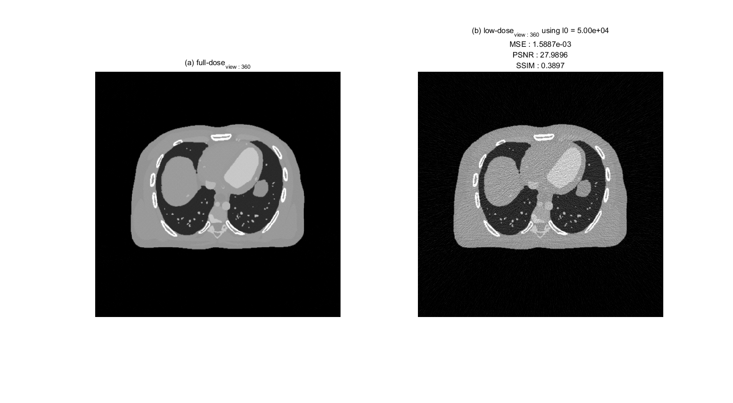
endIn X-ray computed tomography (CT) system, radiation exposure is critical limitation. To reduce the radiation exposure, X-ray CT system uses a low-dose X-ray source. The low-dose X-ray source generate severe poison noise when X-ray photon are measured at X-ray detector, then a reconstruction image using low-dose measurement is too noisy to diagnosis diseases by doctor. Below image shows (a) full-dose image and (b) low-dose image, respectively.
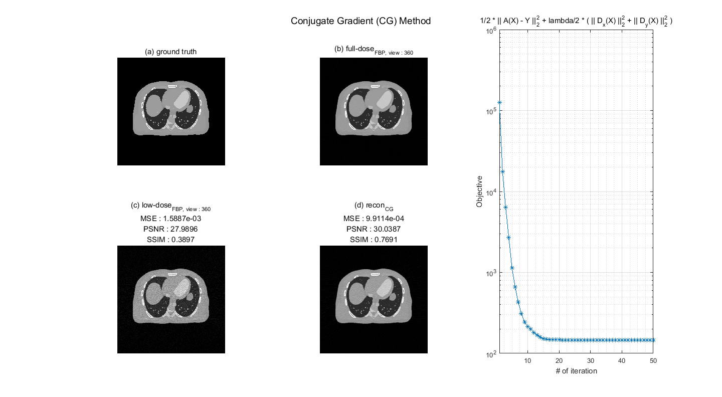
To reduce the noise, objective function with total variation (TV) regularization can be formulated as follows:
where
In above equation, since each terms is quadratic function, an optimal point of
$$A^TA + \lambda( D_x^T D_x + D_y^T D_y) = A^T\textrm{y}.$$
To match the CG formula,
Now, above equation form

