harp-lab/brainPH

Brain Persistent Homology

Using persistent homology and multidimensional scaling on Wasserstein distance matrix

Data pre-processing

Input matrix

• S x C x N x N, where S = #subjects, C = #cohorts, N = #ROIs
• Mat file
• Size: 316 x 3 x 114 x 114
• Three cohorts: mx645, mx1400, std2500

Data normalization

• Removed NaN values by removing column 24 and row 24 from each 114 x 114 matrix
• Used correlation coefficients on transposed matrix and then applied square root on the 1 - squared distance
• 316 x 3 files, 3 files for each subject
• Each file contains 113 x 113 matrix
• Example: subject_1_mx645.txt, subject_1_mx1400.txt, subject_1_std2500.txt

Pipeline 1: Comparison across cohorts

Persistent homology

• Computed 0-dimensional persistent homology (PH) for all three cohorts of each subjects
• Generated 0-dimensional barcodes from calculated PH values with maximum value of 1
• To use persistent homology features from Gudhi library set manual=False in get_barcodes_single_subject method in distance_calculation.py. Otherwise, set manual=True for raw calculation of persistent homology and 0-dimensional barcodes.

Distance calculation

• Computed 1-Wasserstein Distance (WD) between cohorts for each subjects from the 0-dimensional barcodes
• For each subject, computed WD on the 0-dimensional barcodes:
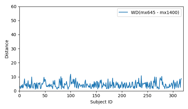
  • WD(mx645 - mx1400)
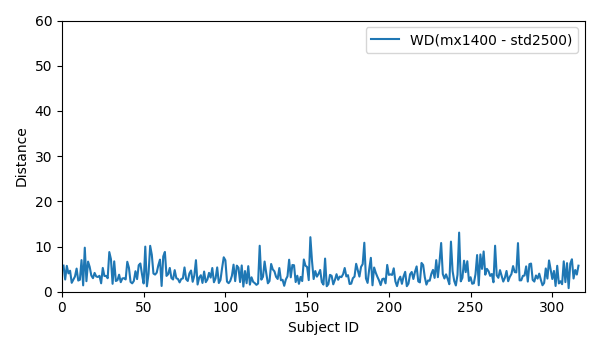
  • WD(mx1400 - std2500)
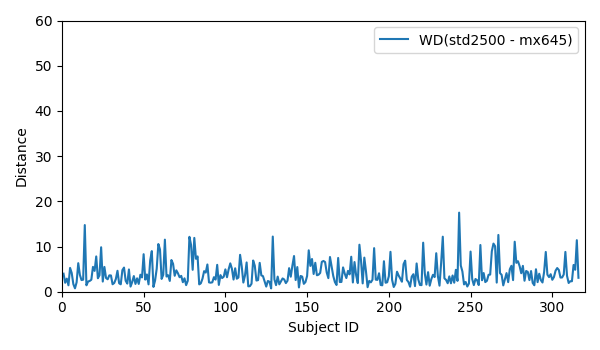
  • WD(std2500 - mx645)
• Generated 1 JSON file with 316 arrays, each array contains 3 values
• Generated file: distances_between_cohorts_ws.json

Pipeline 2: Comparison within a cohort

Persistent homology

• Computed 0-dimensional persistent homology (PH) for all three cohorts of each subjects
• Generated 0-dimensional barcodes from calculated PH values with maximum value of 1
• To use persistent homology features from Gudhi library set manual=False in get_barcodes_single_subject method in distance_calculation.py. Otherwise, set manual=True for raw calculation of persistent homology and 0-dimensional barcodes.

Distance matrix (Wasserstein distance)

• Computed 1-Wasserstein Distance (WD) matrix within a cohort separately
• For each cohort, computed WD distance matrix on the 0-dimensional barcodes:
  • WD_matrix(mx645): 316 x 316
  • WD_matrix(mx1400): 316 x 316
  • WD_matrix(std2500): 316 x 316
• Generated 3 JSON files each with 316 x 316 matrix
• Generated files:
  • distance_matrix_mx645_ws.json
  • distance_matrix_mx1400_ws.json
  • distance_matrix_std2500_ws.json

Multidimensional scaling (Wasserstein distance)

• Applied classical metric Multidimensional scaling (MDS) with precomputed distance (1-Wasserstein)
• Calculated MDS of 2 components for each 1-Wasserstein distance matrix
• Generated 3 JSON files each with 316 x 2 matrix
• Generated files:
  • mds_mx645_ws.json
  • mds_mx1400_ws.json
  • mds_std2500_ws.json
• Applied Kmeans++ clustering by selecting the number of clusters n using Silhouette Coefficient.
  • clustering_ws.json

Statistical analysis

• Calculate p-value using ANOVA test on the [316 x 3] size Wasserstein distances between the cohorts
• ANOVA test p-value: 0.133
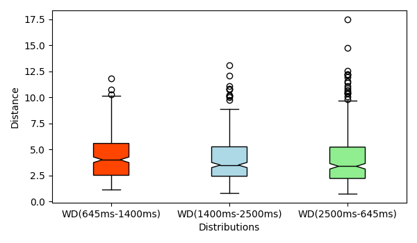
• Wasserstein distance for the following three pairs: (1) TR=645ms and TR=1400ms, (2) TR=1400ms and TR=2500ms and, (1) TR=2500ms and TR=645ms plotted using box plots: boxplots
• Plot WD distances between:
  • WD for all 316 subjects for mx645 and mx1400: WD_mx645_mx1400
  • WD for all 316 subjects for mx1400 and std2500: WD_mx1400_std2500
  • WD for all 316 subjects for std2500 and mx645: WD_std2500_mx645
• Plot MDS value for all three cohorts: mds graph
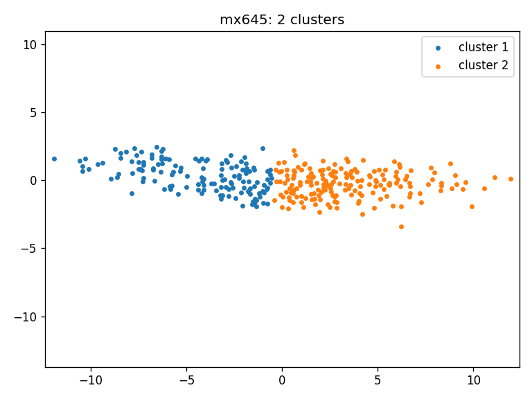
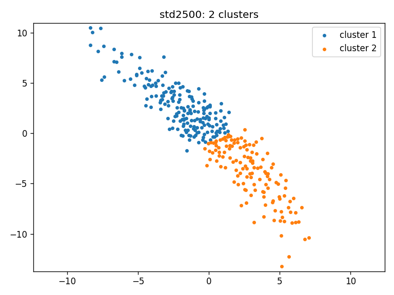
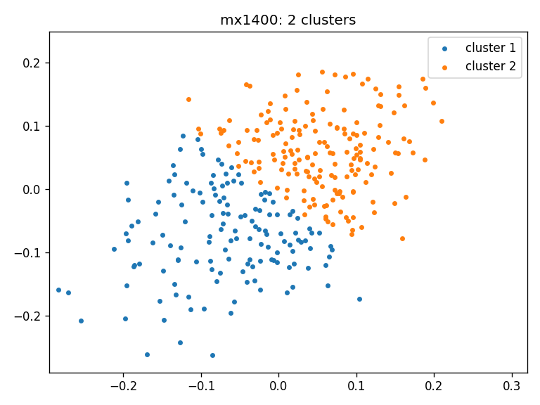
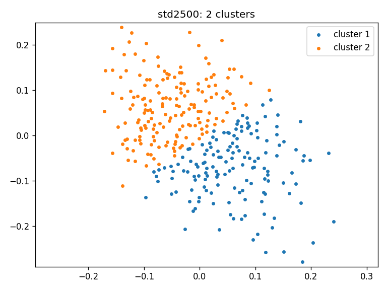
• Clustering on the MDS results
  • Wasserstein distance:
    • Single figure: clustering_ws
    • mx1400: clusters_mx1400_ws
    • mx645: clusters_mx645_ws
    • std2500: clusters_std2500_ws

Local Setup

Requirements

• Python 3

Install dependencies

• Clone the repository.
• Open a terminal / powershell in the cloned repository.
• Create a virtual environment and activate it. If you are using Linux / Mac:

python3 -m venv venv
source venv/bin/activate

Create and activate venv in Windows (Tested in Windows 10):

python -m venv venv
Set-ExecutionPolicy -ExecutionPolicy RemoteSigned -Scope CurrentUser
.\venv\Scripts\Activate.ps1

After activating venv, the terminal / powershell will have (venv) added to the prompt.

• Check pip version:

pip --version

It should point to the pip in the activated venv.

• Install required packages:

pip install -r requirements.txt

Run the project:

• Calculate distance between cohorts and MDS within a cohort using WD:

python distance_calculation.py --method ws --start 1 --end 316 --distance y --mds y --data_dir full_data_linear --output_dir output_linear

• Draw plots and ANOVA test:

python statistical_calculation_linear.py --output_dir output_linear

• Generate clusters on the MDS data:

python cluster_calculation.py --output_dir output_linear

Results

• Generate distance and MDS:

python distance_calculation.py --method ws --start 1 --end 316 --distance y --mds y --data_dir full_data_linear --output_dir output_linear

• Running statistical analysis on the generated file:

python statistical_calculation_linear.py --output_dir output_linear
T-values:
0.059044 0.459634 0.286013 
P-values:
0.088131 0.518936 0.387180 
ANOVA test p-value: 0.289941
Mean WD_MX645_MX1400: 4.304
Mean WD_MX1400_STD2500: 4.01
Mean WD_STD2500_MX645: 4.135
WD_MX645_MX1400: Distance:   2, number of subjects:  42, percentage: 13.29%
WD_MX645_MX1400: Distance:   5, number of subjects: 207, percentage: 65.51%
WD_MX645_MX1400: Distance>  10, number of subjects:   4, percentage: 1.27%
Method main executed in 128.7125 seconds

• T-values and p-values obtained by pairwise t-tests comparing the WDs between data cohorts. Since all p-values are greater than 0.05, the means of WD distributions for each cohort comparison are statistically similar.

		t-value	p-value
WD(P1, P2)	WD(P2, P3)	0.059044	0.088131
WD(P2, P3)	WD(P3, P1)	0.459634	0.518936
WD(P3, P1)	WD(P1, P2)	0.286013	0.387180

• Wasserstein distance for the following three pairs: (1) TR=645ms and TR=1400ms, (2) TR=1400ms and TR=2500ms and, (1) TR=2500ms and TR=645ms plotted using box plots:
• WD for all 316 subjects for mx645 and mx1400:
• WD for all 316 subjects for mx1400 and std2500:
• WD for all 316 subjects for std2500 and mx645:
• Clustering result for all three cohorts using Wasserstein distance:
  • mx1400:
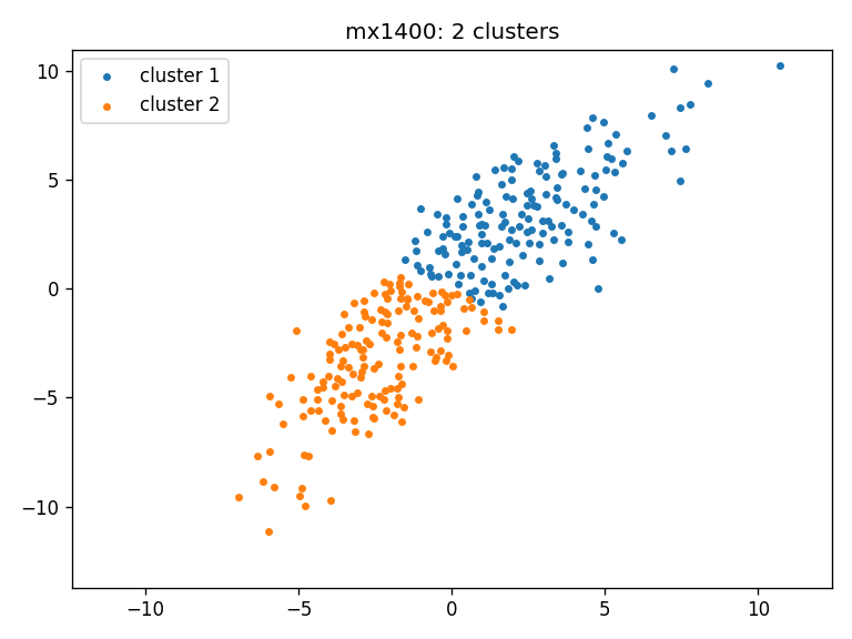
  • mx645:
  • std2500:

Generated files:

• distances_between_cohorts_ws.json
• distance_matrix_mx645_ws.json
• distance_matrix_mx1400_ws.json
• distance_matrix_std2500_ws.json
• mds_mx645_ws.json
• mds_mx1400_ws.json
• mds_std2500_ws.json
• clustering_ws.json

Clustering results (review update)

TDA cluster generation (linear data)

Clustering result (within cohort):

python cluster_calculation.py --output_dir output_linear

Number of clusters in 3 cohorts: [2, 2, 2]
output_linear:
Cluster group: 000: #match: 24
Cluster group: 001: #match: 7
Cluster group: 010: #match: 26
Cluster group: 011: #match: 83
Cluster group: 100: #match: 115
Cluster group: 101: #match: 12
Cluster group: 110: #match: 20
Cluster group: 111: #match: 29

Max + reverse: 115 + 83 = 198

645-1400 : 236
1400-2500 : 251
2500-645 : 225

Adjacency matrix:
output_linear:
Rows X Columns: [645 clusters, 1400 clusters, 2500 clusters]
140 0 31 109 50 90 
0 176 127 49 135 41 
31 127 158 0 139 19 
109 49 0 158 46 112 
50 135 139 46 185 0 
90 41 19 112 0 131 

• Clustering result for full data for all three cohorts using Wasserstein distance:
  • mx645:
  • mx1400:
  • std2500:

Statistical analysis on tda pipeline with linear data (across cohort):

python statistical_calculation_linear.py --output_dir output_linear
T-values:
0.059044 0.459634 0.286013 
P-values:
0.088131 0.518936 0.387180 
ANOVA test p-value: 0.289941

• T-values and p-values obtained by pairwise t-tests comparing the WDs between data cohorts. Since all p-values are larger than 0.05, the means of WD distributions for each cohort comparison are statistically similar.

		t-value	p-value
WD(P1, P2)	WD(P2, P3)	0.059044	0.088131
WD(P2, P3)	WD(P3, P1)	0.459634	0.518936
WD(P3, P1)	WD(P1, P2)	0.286013	0.387180

TDA cluster generation (random data - 1 sample)

Clustering result (within cohort):

python cluster_calculation.py --output_dir output_random
Number of clusters in 3 cohorts: [2, 2, 2]
output_random:
Cluster group: 000: #match: 35
Cluster group: 001: #match: 38
Cluster group: 010: #match: 34
Cluster group: 011: #match: 43
Cluster group: 100: #match: 36
Cluster group: 101: #match: 32
Cluster group: 110: #match: 42
Cluster group: 111: #match: 56

Max + reverse: 56 + 35 = 91

Adjacency matrix:
output_random:
Rows X Columns: [645 clusters, 1400 clusters, 2500 clusters]
150 0 73 77 69 81 
0 166 68 98 78 88 
73 68 141 0 71 70 
77 98 0 175 76 99 
69 78 71 76 147 0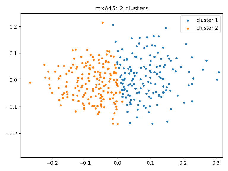 
81 88 70 99 0 169 

• Clustering result for random data for all three cohorts using Wasserstein distance:
  • mx645:
  • mx1400:
  • std2500:

Mean and standard deviation of random clusters (49 out of 50)

Mean value of (Max + Reverse): 84.06122448979592
Standard deviation value of (Max + Reverse): 5.738786759358441

Notes

• Within cohort: clustering
• Across cohorts: statistical analysis
• Original dataset: timeseries.Yeo2011.mm316.mat
• Total negative in correlation coefficient: 1234732 from all_positive_linear.m
• Total positive in correlation coefficient: 10870280 from all_negative_linear.m
• 3 out of 148 random dataset returns cluster 2, 2, 4, 1 returns 4, 2, 2, and 144 returns 2, 2, 2.

To Do:

• non-TDA experiments for within cohort and comparison across cohort
• nonTDA on random for second pipeline
• create two matrices one for positive values and one for negative values and apply the distance function on them. Since, this will be a lot of experiments, if we do this for everything, let us just start by doing with only pipeline 1 (box plots, p/t-value tests). the original mat file which we normalized using matlab. 113 x 113 with all positive (padded by 0) and 113 x 113 with all negative (padded by 0).

References

• Rips complex user manual
• Wasserstein distance user manual
• Bottleneck docs
• ANOVA test using scipy docs
• T-test using scipy docs