Time-Coverage Integrated Plots

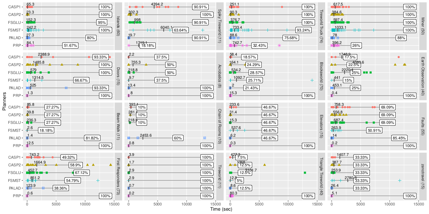
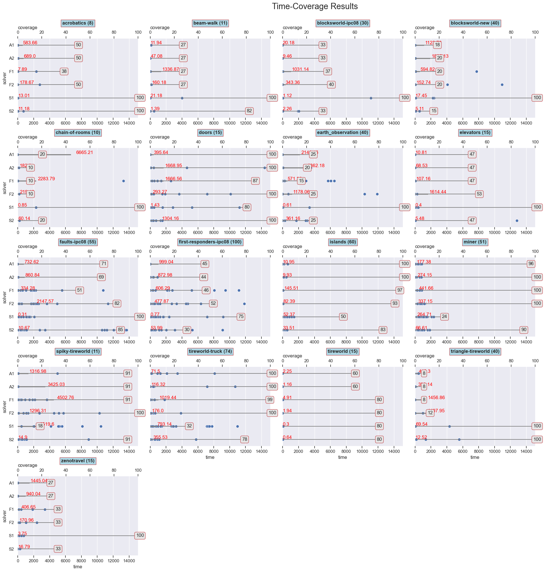
This repo contains R and Python code to produce time-coverage integrated plots for planning experiments, as shown in the following paper:

Nitin Yadav, Sebastian Sardiña: A Declarative Approach to Compact Controllers for FOND Planning via Answer Set Programming. ECAI 2023: 2818-2825

There is one subplot per domain. Each planner shows the coverage % in the domain, and the average time on top of scatter plot of each instance.

CSV data table files

The script require a CSV file containing the following columns:

solver: name of solver (e.g., planner)
domain: name of domain (e.g., blocksworld)
status: integer stating the result of the run, with 1 denoting solved successfully.
solved: boolean stating if run was solved.
cputime: time taken.

Seaborn-based Python plots

Notebook coverage_plots.ipynb plot integrated time-coverage plots using Seaborn Python package.

An example run on data_stats.csv would be:

R plots

The same charts can be produced with Nitin's R script r-plot/plots.R.

Setup

The script requires R.

First make sure you install R-packages dplyr and ggplot2 packages. You can do this from command line once:

$ Rscript -e 'install.packages("dplyr")'
$ Rscript -e 'install.packages("ggplot2")'

Generating plots

First, state the file to read from in plot.R line as well as other configuration parameters under the CONSTANT section:

######################################
#### SET YOUR CONSTANTS
######################################
main_file <- "data_stats"

plot_width <- 15
plot_height <- 12
plot_dpi <- 300

Then, you can use RStudio or simply run from command line:

$ R < plots.R --no-save

This should produce a PDF file and a PNG file with the plots.