Get hands on with Azure Machine Learning (Preview)

Presenters: Heather Shapiro

Introduction and setup

The Primary Concepts for this lab are here. We'll refer to these throughout the lab.

NOTE: These steps must be completed prior to attempting this workshop.

You will need a Microsoft Azure account. You can use a production Azure account if you are able to create objects. You can also use your Microsoft Developer Network (MSDN) account (if you have one) to complete this workshop. If you don't have access to a corporate or MSDN account you can create a free account using this process.
You need to install the Azure Machine Learning Workbench locally. Open this reference and follow the sections marked Install Azure Machine Learning Workbench on Windows or choose your OS type from the instructions there.
This Tutorial is designed to walk you through different combinations of computes and storages to give you a flavor for different scenarios you will encounter in your data-science work:

Scenario	Storage	Compute for Experimentation	Compute for Operationalization	Remarks
1.	Local	Local(python)	Local machine
2.	Azure SQL	DSVM (We will provide)	Local Docker	We will provide Azure SQL access.

You will need
- You will need an Azure Machine Learning Services account. Open this reference, and complete only the sections marked "Sign in to the Azure portal" and "Create Azure Machine Learning accounts". Write down the names of the Experimentation account as well as the Model Management account and bring it to class.
- Docker : Open this reference and follow the instructions for installing Docker locally.
- DSVM: For this tutorial, we will provide you with DSVM credentials. You can create your own by opening this reference and following the instructions for creating a DSVM. For the DSVM choose a VM size of: DS3_V2, with 4 virtual CPUs and 14-Gb RAM. For the HDI cluster choose ClusterType=Spark; OS=Linux and _version=Spark 2.1.0 (HDI 3.6).
- ACR & ACS : Open this reference and follow the instructions under Environment Setup for both Local and Cluster Deployment. Write down the names of the environments you chose and bring it to class.

Step 1: Create an AML account

Create Azure Machine Learning accounts

Use the Azure portal to provision Azure Machine Learning accounts:

Select the New button (+) in the upper-left corner of the portal.
Click the AI + Cognitive Services button under the Azure Marketplace . Select “Machine Learning Experimentation (preview)”. The detailed form will open as seen below.
Fill out the Machine Learning Experimentation form with the following information:

Setting	Suggested value	Description
Experimentation account name	Unique name	Choose a unique name that identifies your account. You can use your own name, or a departmental or project name that best identifies the experiment. The name should be 2 to 32 characters. It should include only alphanumeric characters and the dash (-) character.
Subscription	Your subscription	Choose the Azure subscription that you want to use for your experiment. If you have multiple subscriptions, choose the appropriate subscription in which the resource is billed.
Resource group	Your resource group	You can make a new resource group name, or you can use an existing one from your subscription.
Location	The region closest to your users	Choose the location that's closest to your users and the data resources.
Number of seats	2	Enter the number of seats. This selection affects the pricing. The first two seats are free. Use two seats for the purposes of this Quickstart. You can update the number of seats later as needed in the Azure portal.
Storage account	Unique name	Select Create new and provide a name to create an Azure storage account. Or, select Use existing and select your existing storage account from the drop-down list. The storage account is required and is used to hold project artifacts and run history data.
Workspace for Experimentation account	Unique name	Provide a name for the new workspace. The name should be 2 to 32 characters. It should include only alphanumeric characters and the dash (-) character.
Assign owner for the workspace	Your account	Select your own account as the workspace owner.
Create Model Management account	check	As part of the Experimentation account creation experience, you have the option of also creating the Machine Learning Model Management account. This resource is used when you're ready to deploy and manage your models as real-time web services. We recommend creating the Model Management account at the same time as the Experimentation account.
Account name	Unique name	Choose a unique name that identifies your Model Management account. You can use your own name, or a departmental or project name that best identifies the experiment. The name should be 2 to 32 characters. It should include only alphanumeric characters and the dash (-) character.
Model Management pricing tier	DEVTEST	Select No pricing tier selected to specify the pricing tier for your new Model Management account. For cost savings, select the DEVTEST pricing tier if it's available on your subscription (limited availability). Otherwise, select the S1 pricing tier for cost savings. Click Select to save the pricing tier selection.
Pin to dashboard	check	Select the Pin to dashboard option to allow easy tracking of your Machine Learning Experimentation account on the front dashboard page of the Azure portal.

Select Create to begin the creation process.
On the Azure portal toolbar, click Notifications (bell icon) to monitor the deployment process.

The notification shows Deployment in progress. The status changes to Deployment succeeded when it's done. Your Machine Learning Experimentation account page opens upon success.

Scenario 1: Iris walk-through on Local

Prepare data

Step #1: Create a new project in the Workbench

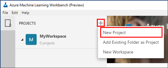
Open the Azure Machine Learning Workbench app, and log in if needed. In the PROJECTS pane, select the plus sign (+) to create a New Project.
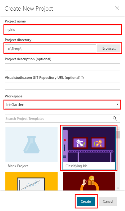
Fill in the Create New Project details:
- Fill in the Project name box with a name for the project. For example, use the value myIris.
- Select the Project directory in which the project is created. For example, use the value C:\Temp\.
- Enter the Project description, which is optional.
- The Git Repository field is also optional and can be left blank. You can provide an existing empty Git repo (a repo with no master branch) on Visual Studio Team Services. If you use a Git repo that already exists, you can enable the roaming and sharing scenarios later. For more information, see Use Git repo.
- Select a Workspace, for example, this tutorial uses IrisGarden.
- Select the Classifying Iris template from the project template list.
Select the Create button. The project is now created and opened for you.

Step #2: Create a data preparation package

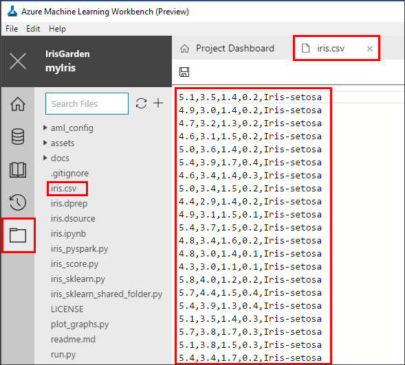
Open the iris.csv file from the File View. The file is a table with 5 columns and 150 rows. It has four numerical feature columns and a string target column. It does not have column headers.
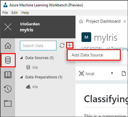
In the Data View, select the plus sign (+) to add a new data source. The Add Data Source page opens.
Leave the default values, and then select the Next button.

Important: Make sure you select the iris.csv file from within the current project directory for this exercise. Otherwise, later steps might fail.

After selecting the file, select the Finish button.
A new file named iris-1.dsource is created. The file is named uniquely with a dash-1, because the sample project already comes with an unnumbered iris.dsource file.

The file opens, and the data is shown. A series of column headers, from Column1 to Column5, is automatically added to this data set. Scroll to the bottom and notice that the last row of the data set is empty. The row is empty because there is an extra line break in the CSV file.

<img src="./media/image8.png" width="647" height="259" />

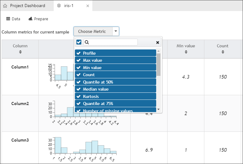
Select the Metrics button. Observe the histograms. A complete set of statistics has been calculated for each column. You can also select the Data button to see the data again.
Select the Prepare button. The Prepare dialog box opens.
- The sample project comes with an iris.dprep file. By default, it asks you to create a new data flow in the iris.dprep data preparation package that already exists.
Select + New Data Preparation Package from the drop-down menu, enter a new value for the package name, use iris-1, and then select OK.
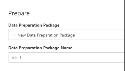
- A new data preparation package named iris-1.dprep is created and opened in the data preparation editor.
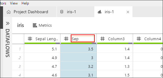
Now let's do some basic data preparation. Rename the column names. Select each column header to make the header text editable.
- Enter Sepal Length, Sepal Width Petal Length, Petal Width and Species for the five columns respectively.
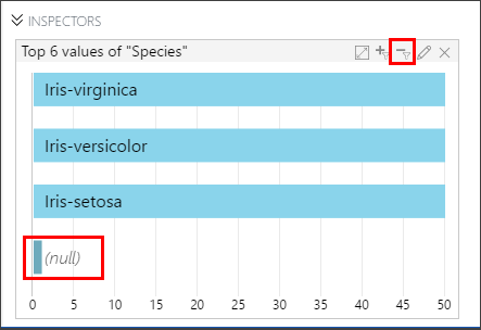
To count distinct values, select the Species column, and then right-click to select it. Select Value Counts from the drop-down menu.
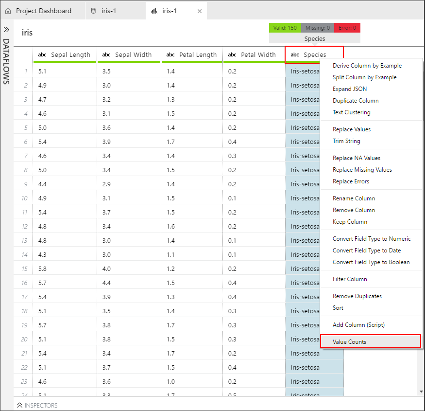
- This action opens the Inspectors pane, and displays a histogram with four bars. The target column has three distinct values: Iris_virginica, Iris_versicolor, Iris-setosa, and a (null) value.
To filter out nulls, select the bar from the graph that represents the null value. There is one row with a (null)value. To remove this row, select the minus sign (-).
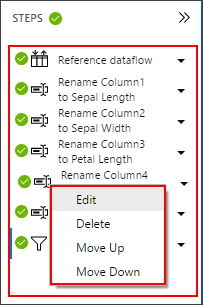
Notice the individual steps detailed in the STEPS pane. As you renamed the columns and filtered the null value rows, each action was recorded as a data-preparation step. You can edit individual steps to adjust the settings, reorder the steps, and remove steps.
Close the data preparation editor. Select Close (x) on the iris-1 tab with the graph icon. Your work is automatically saved into the iris-1.dprep file shown under the Data Preparations heading.

Step #3: Generate Python/PySpark code to invoke a data preparation package

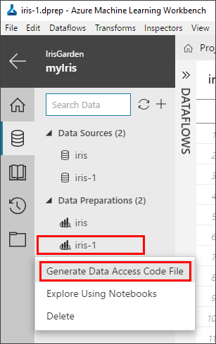
Right-click the iris-1.dprep file to bring up the context menu, and then select Generate Data Access Code File.
A new file named iris-1.py opens with the following lines of code:

# Use the Azure Machine Learning data preparation package

from azureml.dataprep import package

# Use the Azure Machine Learning data collector to log various
metrics

from azureml.logging import get\_azureml\_logger

logger = get\_azureml\_logger()

# This call will load the referenced package and return a DataFrame.
# If run in a PySpark environment, this call returns a

# Spark DataFrame. If not, it will return a Pandas DataFrame.

df = package.run('iris-1.dprep', dataflow\_idx=0)

# Remove this line and add code that uses the DataFrame

df.head(10)

This code snippet invokes the logic you created as a data preparation package. Depending on the context in which this code is run, df represents the various kinds of dataframes. A pandas DataFrame is used when executed in Python runtime, or a Spark DataFrame is used when executed in a Spark context.
For more information on how to prepare data in Azure Machine Learning Workbench, see the Get started with data preparation guide.

Build a model

Step #1: Review iris_sklearn.py and the configuration files

Select the Files button (the folder icon) on the far-left pane to open the file list in your project folder.
Select the iris_sklearn.py file. The Python code opens in a new text editor tab inside the workbench.
Review the Python script code to become familiar with the coding style. The script performs the following tasks:
- Loads the data preparation package iris.dprep to create a pandas DataFrame.

Note

Use the iris.dprep data preparation package that comes with the sample project, which should be the same as the iris-1.dprep file you built in part 1 of this tutorial.

Adds random features to make the problem more difficult to solve. Randomness is necessary because Iris is a small data set that's easily classified with nearly 100% accuracy.
Uses the scikit-learn machine learning library to build a logistic regression model.
Serializes the model by inserting the pickle library into a file in the outputs folder. The script then loads it and deserializes it back into memory.
Uses the deserialized model to make a prediction on a new record.
Plots two graphs, a confusion matrix and a multi-class receiver operating characteristic (ROC) curve, by using the matplotlib library, and then saves them in the outputs folder.
The run_logger object is used throughout to record the regularization rate and to model accuracy into the logs. The logs are automatically plotted in the run history.

Step #2: Execute iris_sklearn.py script in a local environment

Let's prepare to run the iris_sklearn.py script for the first time. This script requires the scikit-learn and matplotlib packages. The scikit-learn package is already installed by Azure Machine Learning Workbench. You still need to install matplotlib.

In Azure Machine Learning Workbench, select the File menu, and then select Open Command Prompt to open the command prompt.

The command-line interface window is referred to as the Azure Machine Learning Workbench CLI window, or CLI window for short.
In the CLI window, enter the following command to install the matplotlib Python package. It should finish in less than a minute.

pip install matplotlib

Note

If you skip the previous pip install command, the code in iris_sklearn.py runs successfully. If you only run iris_sklearn.py, the code doesn't produce the confusion matrix output and the multi-class ROC curve plots as shown in the history visualizations.
Return to the workbench app window.
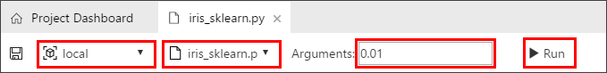
In the toolbar at the top of the iris_sklearn.py tab, select to open the drop-down menu that is next to the Save icon, and then select Run Configuration. Select local as the execution environment, and then enter iris_sklearn.py as the script to run.
Next, move to the right side of the toolbar and enter 0.01 in the Arguments field.
Select the Run button. A job is immediately scheduled. The job is listed in the Jobs pane on the right side of the workbench window.
After a few moments, the status of the job transitions from Submitting, to Running, and then to Completed.
Select Completed in the job status text in the Jobs pane. A pop-up window opens and displays the standard output (stdout) text of the running script. To close the stdout text,select the Close (x) button on the upper right of the pop-up window.
In the same job status in the Jobs pane, select the blue text iris_sklearn.py [n] (n is the run number) just above the Completed status and the start time. The Run Properties window opens and shows the following information for that particular run:
- Run Properties information
- Outputs files
- Visualizations, if any
- Logs

When the run is finished, the pop-up window shows the following results:

Note

Because we introduced some randomization into the training set earlier, your exact results might vary from the results shown here.

Python version: 3.5.2 |Continuum Analytics, Inc.| (default, Jul  5 2016, 11:41:13) [MSC v.1900 64 bit (AMD64)]

Iris dataset shape: (150, 5)
Regularization rate is 0.01
LogisticRegression(C=100.0, class_weight=None, dual=False, fit_intercept=True,
       intercept_scaling=1, max_iter=100, multi_class='ovr', n_jobs=1,
       penalty='l2', random_state=None, solver='liblinear', tol=0.0001,
       verbose=0, warm_start=False)
Accuracy is 0.6792452830188679

==========================================
Serialize and deserialize using the outputs folder.

Export the model to model.pkl
Import the model from model.pkl
New sample: [[3.0, 3.6, 1.3, 0.25]]
Predicted class is ['Iris-setosa']
Plotting confusion matrix...
Confusion matrix in text:
[[50  0  0]
 [ 1 37 12]
 [ 0  4 46]]
Confusion matrix plotted.
Plotting ROC curve....
ROC curve plotted.
Confusion matrix and ROC curve plotted. See them in Run History details pane.

Close the Run Properties tab, and then return to the iris_sklearn.py tab.
Repeat additional runs.
- Enter a series of different numerical values in the Arguments field ranging from 0.001 to 10. Select Run to execute the code a few more times. The argument value you change each time is fed to the logistic regression algorithm in the code, and that results in different findings each time.

Step #3: Review the run history in detail

In Azure Machine Learning Workbench, every script execution is captured as a run history record. If you open the Runs view, you can view the run history of a particular script.

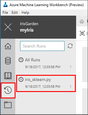
To open the list of Runs, select the Runs button (clock icon) on the left toolbar. Then select iris_sklearn.py to show the Run Dashboard of iris_sklearn.py.
The Run Dashboard tab opens. Review the statistics captured across the multiple runs. Graphs render in the top of the tab. Each run has a consecutive number, and the run details are listed in the table at the bottom of the screen.
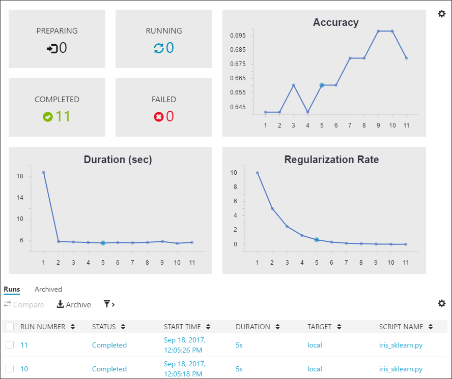
Filter the table, and then select any of the graphs to view the status, duration, accuracy, and regularization rate of each run.
Select two or three runs in the Runs table, and select the Compare button to open a detailed comparison pane. Review the side-by-side comparison. Select the Run List back button on the upper left of the Comparison pane to return to the Run Dashboard.
Select an individual run to see the run detail view. Notice that the statistics for the selected run are listed in the Run Properties section. The files written into the output folder are listed in the Outputs section, and you can download the files from there.

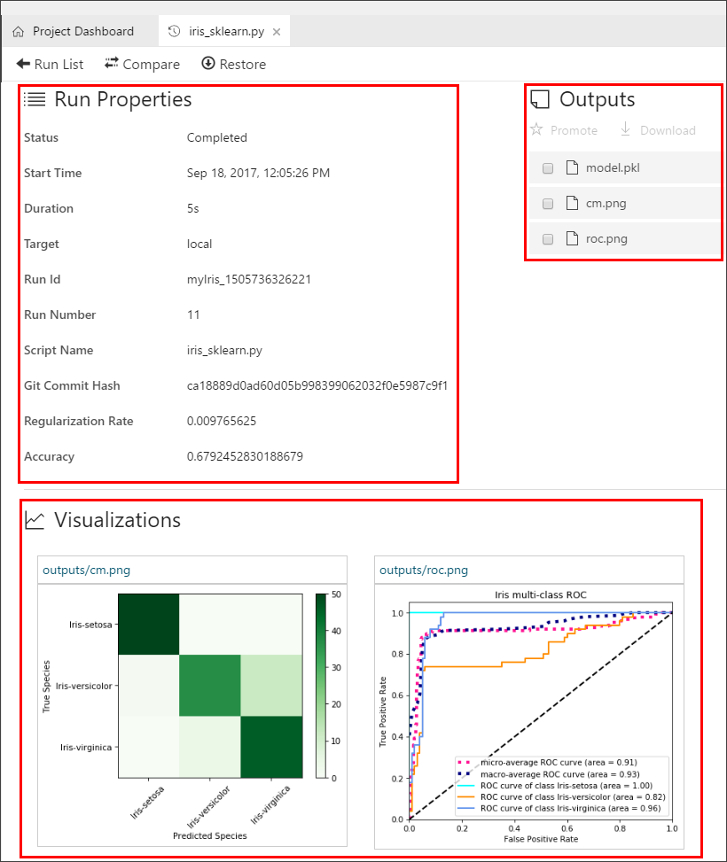
The two plots, the confusion matrix and the multi-class ROC curve, are rendered in the Visualizations section. All the log files can also be found in the Logs section.

Deploy a model

Step #1: Download the model pickle file

In the previous part of the tutorial,the iris_sklearn.py script was run in Machine Learning Workbench locally. That action serialized the logistic regression model by using the popular Python object-serialization package pickle.

Open the Machine Learning Workbench application, and then open the myIris project you created in the previous part of the tutorial series.
After the project is open, select the Files button (folder icon) on the left pane to open the file list in your project folder.
Select the iris_sklearn.py file. The Python code opens in a new text editor tab inside the workbench.
Review the iris_sklearn.py file to see where the pickle file was generated. Select Ctrl+F to open the Finddialog box, and then find the word pickle in the Python code.
- This code snippet shows how the pickle output file was generated. The output pickle file is named model.pkl on the disk.
```
print("Export the model to model.pkl")
f = open('./outputs/model.pkl', 'wb') pickle.dump(clf1, f)
f.close()
```
Locate the model pickle file in the output files of a previous run.

When you ran the iris_sklearn.py script, the model file was written to the outputs folder with the name model.pkl. This folder lives in the execution environment that you choose to run the script, and not in your local project folder.
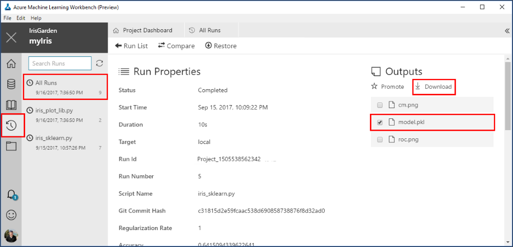
- To locate the file, select the Runs button (clock icon) on the left pane to open the list of All Runs.
- The All Runs tab opens. In the table of runs, select one of the recent runs where the target was local and the script name was iris_sklearn.py.
- The Run Properties pane opens. In the upper-right section of the pane, notice the Outputs section.
- To download the pickle file, select the check box next to the model.pkl file, and then select the Download button. Save it to the root of your project folder. The file is needed in the upcoming steps.

Step #2: Get the scoring script and schema files

To deploy the web service along with the model file, you also need a scoring script, and optionally, a schema for the web-service input data. The scoring script loads the model.pkl file from the current folder and uses it to produce a newly predicted Iris class.

Select the Files button (folder icon) on the left pane to open the file list in your project folder.
Select the score_iris.py file. The Python script opens. This file is used as the scoring file.
To get the schema file, run the script. Select the local environment and the score_iris.py script in the command bar, and then select the Run button.
This script creates a JSON file in the Outputs section, which captures the input data schema required by the model.
Note the Jobs pane on the right side of the Project Dashboard pane. Wait for the latest score_iris.py job to display the green Completed status. Then select the hyperlink score_iris.py [1] for the latest job run to see the run details from the score_iris.py run.
On the Run Properties pane, in the Outputs section, select the newly created service_schema.json file. Select the check box next to the file name, and then select Download. Save the file into your project root folder.
Return to the previous tab where you opened the score_iris.py script. By using data collection, you can capture model inputs and predictions from the web service. The following steps are of particular interest for data collection.
Review the code at the top of the file imports class ModelDataCollector, because it contains the model data collection functionality:

from azureml.datacollector import ModelDataCollector
Review the following lines of code in the init() function that instantiates ModelDataCollector:

global inputs_dc, prediction_dc
inputs_dc = ModelDataCollector('model.pkl',identifier="inputs")
prediction_dc = ModelDataCollector('model.pkl', identifier="prediction")`

Review the following lines of code in the run(input_df) function as it collects the input and prediction data:

global clf2, inputs_dc, prediction_dc
inputs_dc.collect(input_df)
prediction_dc.collect(pred)

Now you're ready to prepare your environment to operationalize the model.

Step #3: Prepare to operationalize locally

Use local mode deployment to run in Docker containers on your local computer.

You can use local mode for development and testing. The Docker engine must be run locally to complete the following steps to operationalize the model. You can use the -h flag at the end of the commands for command Help.

Note

If you don't have the Docker engine locally, you can still proceed by creating a cluster in Azure for deployment. Just be sure to delete the cluster after the tutorial so you don't incur ongoing charges.

Open the command-line interface (CLI). In the Azure Machine Learning Workbench application, on the File menu, select Open Command Prompt. The command-line prompt opens in your current project folder location c:\temp\myIris>.
Make sure you are logged in with az login

Make sure the Azure resource provider Microsoft.ContainerRegistry is registered in your subscription. You must register this resource provider before you can create an environment in step 3. You can check to see if it's already registered by using the following command:

az provider list
--query "[].{Provider:namespace, Status:registrationState}"
--out table

Provider Status
-------- ------
Microsoft.Authorization Registered

Microsoft.ContainerRegistry Registered

microsoft.insights Registered

Microsoft.MachineLearningExperimentation Registered

If Microsoft.ContainerRegistry is not registered, you can register it by using the following command: az provider register --namespace Microsoft.ContainerRegistry

Registration can take a few minutes. You can check on its status by using the previous az provider list command or az provider show -n Microsoft.ContainerRegistry

The third line of the output displays **"registrationState":

"Registering"**. Wait a few moments and repeat the **show** command until the output displays **"registrationState": "Registered"**.

Create the environment. You must run this step once per environment.
- For example, run it once for development environment, and once for production. Use local mode for this first environment. You can try the -c or --cluster switch in the following command to set up an environment in cluster mode later.
- Note that the following setup command requires you to have Contributor access to the subscription. If you don't have that, you at least need Contributor access to the resource group that you are deploying into. To do the latter, you need to specify the resource group name as part of the setup command using -g the flag.
az ml env setup -n <new deployment environment name> --location <e.g. eastus2>

Follow the on-screen instructions to provision a storage account for storing Docker images, an Azure container registry that lists the Docker images, and an AppInsight account that gathers telemetry. If you used the -c switch, it creates an Azure Container Service cluster too.

The cluster name is a way for you to identify the environment. The location should be the same as the location of the Model Management account you created from the Azure portal.

Create a Model Management account. (This is a one-time setup.)

az ml account modelmanagement create --location <e.g. eastus2> -n <new model management account name> -g <existing resource group name> --sku-name S1
Set the Model Management account.

az ml account modelmanagement set -n <youracctname> -g <yourresourcegroupname>
Set the environment.

After the setup finishes, use the following command to set the environment variables required to operationalize the environment. Use the same environment name that you used previously in step 4. Use the same resource group name that was output in the command window when the setup process finished.

az ml env set -n <deployment environment name> -g <existing resource group name>

To verify that you have properly configured your operationalized environment for local web service deployment, enter the following command:

az ml env show

Now you're ready to create the real-time web service.

Note

You can reuse your Model Management account and environment for subsequent web service deployments. You don't need to create them for each web service. An account or an environment can have multiple web services associated with it.

Step #4: Create a real-time web service in one command

To create a real-time web service, use the following command:

az ml service create realtime -f score\_iris.py --model-file model.pkl -s service\_schema.json -n irisapp -r python --collect-model-data true

This command generates a web service ID you can use later.

The following switches are used with the az ml service create realtime command:
- -n: The app name, which must be all lowercase.
- -f: The scoring script file name.
- --model-file: The model file. In this case, it's the pickled model.pkl file.
- -r: The type of model. In this case, it's a Python model.
- --collect-model-data true: This enables data collection.

Important

The service name, which is also the new Docker image name, must be all lowercase. Otherwise, you get an error.

When you run the command, the model and the scoring file upload to the storage account you created as part of the environment setup.The deployment process builds a Docker image with your model, schema, and scoring file in it, and then pushes it to the Azure container registry: <ACR_name>.azureacr.io/<imagename>:<version>.

The command pulls down the image locally to your computer, and then starts a Docker container based on that image. If your environment is configured in cluster mode, the Docker container is deployed into the Azure Cloud Services Kubernetes cluster instead.

As part of the deployment, an HTTP REST endpoint for the web service is created on your local machine. After a few minutes, the command should finish with a success message and your web service is ready for action.

To see the running Docker container, use the docker ps command:

docker ps

Step #5: Run the real-time web service

To test the irisapp web service that's running, use a JSON-encoded record containing an array of four random numbers:

The web service includes sample data. When running in local mode, you can call the az ml service usage realtime command. That call retrieves a sample run command that's useful for you to use to test the service. The call also retrieves the scoring URL that you can use to incorporate the service into your own custom app:

az ml service usage realtime -i <service ID>
To test the service, execute the returned service run command:

az ml service run realtime -i irisapp -d "{\"input_df\": [{\"petal width\": 0.25, \"sepal length\": 3.0, \"sepal width\": 3.6, \"petal length\": 1.3}]}"

The output is "2", which is the predicted class. (Your result might be different.)

To run the service from outside the CLI, you need to get the keys for authentication:

az ml service keys realtime -i <web service ID>

Scenario#2: Change the Data Source to SQL Server and Experimentation Compute Target to a DSVM

In this scenario, we will learn how to change the data source for an existing data flow within a preparation package.

Change the Data Source to Azure SQL:

This part assumes that you have the iris data loaded to an Azure SQL DB.

You can use the following script to create the iris table, and then use SSMS or another tool to upload iris.csv to the table.

CREATE TABLE \[dbo\].\[iris\](

\[Sepal Length\] \[varchar\](50) NULL,

\[Sepal Width\] \[varchar\](50) NULL,

\[Petal Length\] \[varchar\](50) NULL,

\[Petal Width\] \[varchar\](50) NULL,

\[Species\] \[varchar\](50) NULL

)

Ensure that Azure SQL DB Firewall allows connection from your IP address.

You will need to whitelist your public IP Address

Create a new Data Source in the workbench by connecting to the Azure DB.

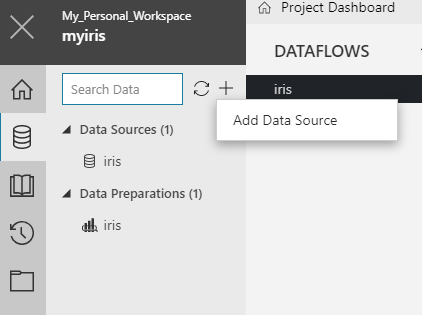
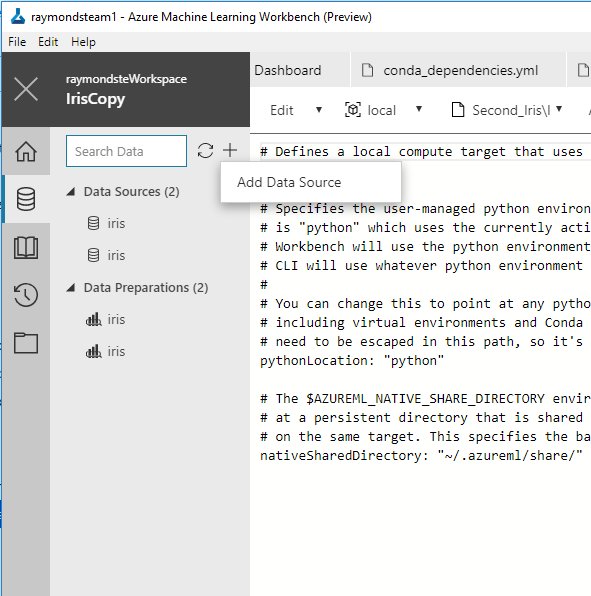
Click on Add Data Source from the Data Tab:

Select Database from the supported data stores, and provide connection details as well as the query to read from the database:

You may click on Preview to see the data.

Click Next, select the default sampling scheme

Click Finish.

A new data source has been created. Note the name of the dataflow created. You will need to use that in the next step.

Normally – You could just change the datasource in the local runconfig.

You can substitute the datasource in the runconfig file. You will have one runconfig file per environment. In this step, we will do the substitution in the local runconfig file.

Open the local.runconfig file by clicking on local.runconfig from the Files tab

Go to the edit mode by clicking on ‘Edit as text in Workbench’

Add the following lines to the local.runconfig and save it. If you named your data source differently, use the appropriate name.

Run the iris_sklearn.py file on the local compute environment

Click on the Run button to execute the python script in the local compute environment. A job should get created and executed.

However it fails because we have to do some data prep first with the SQL computefest database.

Click the computefest datasource and select Prepare

Notice that the columns are listed as strings instead of numbers. We can change that by deriving a column by example. Right click on the Sepal Length column and select Derive Column by Example

Type 5.1.

Notice that the rest of the column should autofill. Select OK and click the # sign to convert the column to numeric. Now repeat this step for Sepal Width, Petal Length, and Petal Width.

Delete the duplicate columns.

Rename the new numeric columns.

Don’t forget to remove the null column at the end like we did earlier!

We can now go change the dprep file in the iris_sklearn.py file and run.

Change the Compute Target to DSVM:

In the previous step we learned how to change the data source for an existing data flow within a data preparation package. In this step, we will learn how to run your scripts on an Azure DSVM from the workbench.

We will use an already provisions DSVM. See this link for provisioning a DVSM of your own: https://docs.microsoft.com/en-us/azure/machine-learning/preview/how-to-create-dsvm-hdi

Open the command prompt from the file menu of the Azure ML Workbench. Then, attach the DSVM compute target using the following command. Give a compute target name you want to use.

az ml computetarget attach remotedocker --name <compute target name> --address <ip address or FQDN> --username <admin username> --password <admin password>

It may take 5-10 minutes.
Run the following command to prepare the Docker image of the DSVM

az ml experiment prepare -c <compute target name>

It may take another 10 minutes to complete.
Select the new compute target from the dropdown in the header and click Run. A job should get created. This time, the data is being fetched from the SQL server and the experimentation is being executed on the Azure DSVM.

Scenario#3: Read Data from Blob Store, run experiment on HDI Cluster and Operationalize to ACS – TO DO ON YOUR OWN

Connect to Blob Storage:

This assumes that your iris.csv file is stored at the Azure blob store.

Create a new data source:
1. Click the Data button (cylinder icon) on the left toolbar. This displays the Data View.
2. Select the + icon and then select Add Data Source.
3. Select ‘Files/Directory’ and click ‘Next’
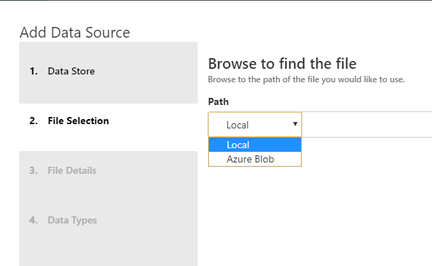
4. Click the down arrow in the ‘Path’ box and select ‘Azure Blob’
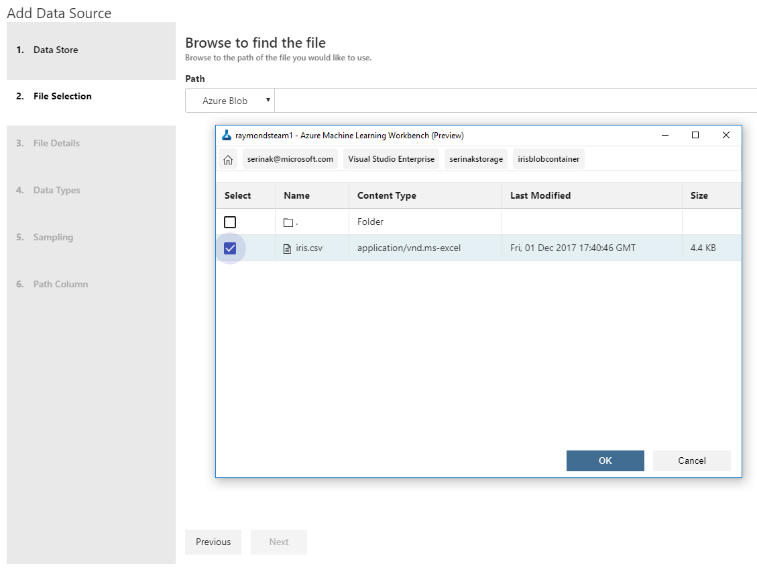
5. Click ‘Browse’ and select the Azure Subscription you’d like to use.
6. Click the Azure Storage account you’d like to use.
7. Selected the container and file you’d like to use.
8. Click ‘Next’ – it is ok to accept all the defaults.
9. After selecting the file, select the Finish button.
10. A new file named iris-1.dsource (or something similar) is created. The file is named uniquely with a dash-1, because the sample project already comes with an unnumbered iris.dsource file.

Create an HDInsight Cluster and Run Your Experiment

Create the cluster - To run scale-out Spark jobs, you need to create an Apache Spark for Azure HDInsight cluster in Azure portal.
- Log on to Azure portal from https://portal.azure.com
- Click on the +NEW link, and search for "HDInsight".
- Choose HDInsight in the list, and then click on the Create button.
- In the Basics configuration screen, Cluster type settings, make sure you choose Spark as the Cluster type, Linux as the Operating system, and Spark 2.1.0 (HDI 3.6) as the _Version.
- Choose the cluster size and node size you need and finish the creation wizard. It can take up to 30 minutes for the cluster to finish provisioning.
Attach the HDI Spark cluster as a compute target - Once the Spark HDI cluster is created, you can now attach it to your Azure ML project.
Substitute the data source in the corresponding runconfig file: Add the following lines to the runconfig file:

DataSourceSubstitutions:

iris.dsource: <new data source name>.dsource

Run the experiment on the cluster - Run the following command, and the script runs in the HDInsight cluster:

Operationalize Your Model with Azure Container Service

Download the model pickle file - Locate the model pickle file in the output files of a previous run. When you ran the iris_sklearn.py script, the model file was written to the outputs folder with the name model.pkl. This folder lives in the execution environment that you choose to run the script, and not in your local project folder.
- To locate the file, select the Runs button (clock icon) on the left pane to open the list of All Runs.
- The All Runs tab opens. In the table of runs, select one of the recent runs where the target was local and the script name was iris_sklearn.py.
- The Run Properties pane opens. In the upper-right section of the pane, notice the Outputs section.
- To download the pickle file, select the check box next to the model.pkl file, and then select the Download button. Save it to the root of your project folder. The file is needed in the upcoming steps.
Get the scoring script and schema files - To deploy the web service along with the model file, you also need a scoring script, and optionally, a schema for the web-service input data. The scoring script loads the model.pkl file from the current folder and uses it to produce a newly predicted Iris class.
- Select the score_iris.py file. The Python script opens. This file is used as the scoring file.
- To get the schema file, run the script.
  - Select the local environment and the score_iris.py script in the command bar, and then select the Run button. This script creates a JSON file in the Outputs section, which captures the input data schema required by the model.
    
    Note the Jobs pane on the right side of the Project Dashboard pane. Wait for the latest score_iris.py job to display the green Completed status. Then select the hyperlink score_iris.py [1] for the latest job run to see the run details from the score_iris.py run.
- On the Run Properties pane, in the Outputs section, select the newly created service_schema.json file. Select the check box next to the file name, and then select Download. Save the file into your project root folder.
Ensure your subscription is registered with Azure Container Registry – Make sure the Azure resource provider Microsoft.ContainerRegistry is registered in your subscription. You must register this resource provider before you can create an environment.
**Create and set your model management account - **
Register the environment – To start the setup process, you need to register the environment provider by entering the following command:
Setup and then set the environment - Use Cluster deployment for high-scale production scenarios. It sets up an ACS cluster with Kubernetes as the orchestrator. The ACS cluster can be scaled out to handle larger throughput for your web service calls. The resource group, storage account, and ACR are created quickly. The ACS deployment can take up to 20 minutes.

A resource group (if not provided, or if the name provided does not exist)

A storage account
An Azure Container Registry (ACR)
A Kubernetes deployment on an Azure Container Service (ACS) cluster
An Application insights account

Deploy - You are now ready to deploy your saved model as a web service.
Test the service - Use the following command to get information on how to call the service:+

Addendum, if needed - Creating an Azure Blob Storage Account:

Go to Azure portal
Select “+ Create a Resource’
Type in ‘blob storage’
Follow instructions on screen and deploy
Once service has been deployed, create a new container for Iris data:
1. From Blob service, choose ‘+ Container’
2. Name your new container, e.g. iriscontainer
3. Accept defaults and click ‘OK’
Click on new container
Find the iris.csv file on your hard drive and upload it to blob storage

heatherbshapiro/Workbench-Tutorial