vectorbt allows you to easily backtest strategies with a couple of lines of Python code.
- Here is how much profit we would have made if we invested $100 into Bitcoin in 2014:
import vectorbt as vbt

price = vbt.YFData.download('BTC-USD').get('Close')

pf = vbt.Portfolio.from_holding(price, init_cash=100)
pf.total_profit()
8961.008555963961
- Buy whenever 10-day SMA crosses above 50-day SMA and sell when opposite:
fast_ma = vbt.MA.run(price, 10)
slow_ma = vbt.MA.run(price, 50)
entries = fast_ma.ma_crossed_above(slow_ma)
exits = fast_ma.ma_crossed_below(slow_ma)

pf = vbt.Portfolio.from_signals(price, entries, exits, init_cash=100)
pf.total_profit()
16423.251963801864
- Generate 1,000 strategies with random signals and test them on BTC and ETH:
import numpy as np

symbols = ["BTC-USD", "ETH-USD"]
price = vbt.YFData.download(symbols, missing_index='drop').get('Close')

n = np.random.randint(10, 101, size=1000).tolist()
pf = vbt.Portfolio.from_random_signals(price, n=n, init_cash=100, seed=42)

mean_expectancy = pf.trades.expectancy().groupby(['randnx_n', 'symbol']).mean()
fig = mean_expectancy.unstack().vbt.scatterplot(xaxis_title='randnx_n', yaxis_title='mean_expectancy')
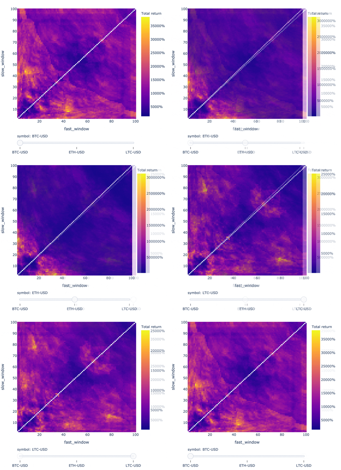
fig.show()- For fans of hyperparameter optimization: here is a snippet for testing 10,000 window combinations of a dual SMA crossover strategy on BTC, USD, and LTC:
symbols = ["BTC-USD", "ETH-USD", "LTC-USD"]
price = vbt.YFData.download(symbols, missing_index='drop').get('Close')

windows = np.arange(2, 101)
fast_ma, slow_ma = vbt.MA.run_combs(price, window=windows, r=2, short_names=['fast', 'slow'])
entries = fast_ma.ma_crossed_above(slow_ma)
exits = fast_ma.ma_crossed_below(slow_ma)

pf_kwargs = dict(size=np.inf, fees=0.001, freq='1D')
pf = vbt.Portfolio.from_signals(price, entries, exits, **pf_kwargs)

fig = pf.total_return().vbt.heatmap(
    x_level='fast_window', y_level='slow_window', slider_level='symbol', symmetric=True,
    trace_kwargs=dict(colorbar=dict(title='Total return', tickformat='%')))
fig.show()
Digging into each strategy configuration is as simple as indexing with pandas:
pf[(10, 20, 'ETH-USD')].stats()Start 2015-08-07 00:00:00+00:00
End 2021-08-01 00:00:00+00:00
Period 2183 days 00:00:00
Start Value 100.0
End Value 620402.791485
Total Return [%] 620302.791485
Benchmark Return [%] 92987.961948
Max Gross Exposure [%] 100.0
Total Fees Paid 10991.676981
Max Drawdown [%] 70.734951
Max Drawdown Duration 760 days 00:00:00
Total Trades 54
Total Closed Trades 53
Total Open Trades 1
Open Trade PnL 67287.940601
Win Rate [%] 52.830189
Best Trade [%] 1075.803607
Worst Trade [%] -29.593414
Avg Winning Trade [%] 95.695343
Avg Losing Trade [%] -11.890246
Avg Winning Trade Duration 35 days 23:08:34.285714286
Avg Losing Trade Duration 8 days 00:00:00
Profit Factor 2.651143
Expectancy 10434.24247
Sharpe Ratio 2.041211
Calmar Ratio 4.6747
Omega Ratio 1.547013
Sortino Ratio 3.519894
Name: (10, 20, ETH-USD), dtype: object
The same for plotting:
pf[(10, 20, 'ETH-USD')].plot().show()It's not all about backtesting - vectorbt can be used to facilitate financial data analysis and visualization.
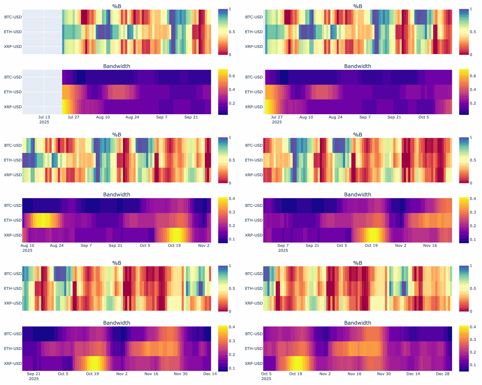
- Let's generate a GIF that animates the %B and bandwidth of Bollinger Bands for different symbols:
symbols = ["BTC-USD", "ETH-USD", "ADA-USD"]
price = vbt.YFData.download(symbols, period='6mo', missing_index='drop').get('Close')
bbands = vbt.BBANDS.run(price)

def plot(index, bbands):
    bbands = bbands.loc[index]
    fig = vbt.make_subplots(
        rows=2, cols=1, shared_xaxes=True, vertical_spacing=0.15,
        subplot_titles=('%B', 'Bandwidth'))
    fig.update_layout(template='vbt_dark', showlegend=False, width=750, height=400)
    bbands.percent_b.vbt.ts_heatmap(
        trace_kwargs=dict(zmin=0, zmid=0.5, zmax=1, colorscale='Spectral', colorbar=dict(
            y=(fig.layout.yaxis.domain[0] + fig.layout.yaxis.domain[1]) / 2, len=0.5
        )), add_trace_kwargs=dict(row=1, col=1), fig=fig)
    bbands.bandwidth.vbt.ts_heatmap(
        trace_kwargs=dict(colorbar=dict(
            y=(fig.layout.yaxis2.domain[0] + fig.layout.yaxis2.domain[1]) / 2, len=0.5
        )), add_trace_kwargs=dict(row=2, col=1), fig=fig)
    return fig

vbt.save_animation('bbands.gif', bbands.wrapper.index, plot, bbands, delta=90, step=3, fps=3)
100%|██████████| 31/31 [00:21<00:00, 1.21it/s]
And this is just the tip of the iceberg of what's possible. Check out the website to learn more.
pip install -U vectorbtTo also install optional dependencies:
pip install -U "vectorbt[full]"All the active development has moved to vectorbt PRO.
This project is being maintained only. PRs are welcome.
This work is fair-code distributed under Apache 2.0 with Commons Clause license. The source code is open and everyone (individuals and organizations) can use it for free. However, it is not allowed to sell products and services that are mostly just this software.
If you have any questions about this or want to apply for a license exception, please contact the author.
Installing optional dependencies may be subject to a more restrictive license.
This software is for educational purposes only. Do not risk money which you are afraid to lose. USE THE SOFTWARE AT YOUR OWN RISK. THE AUTHORS AND ALL AFFILIATES ASSUME NO RESPONSIBILITY FOR YOUR TRADING RESULTS.


