Alberto Villagómez Vargas, Hermes Espínola González, Humberto Atondo Martín del Campo
In this article, we do clustering analysis using an evolutionary optimization algorithm based on nature, Forest Optimization Algorithm (FOA), perfect for continuous nonlinear optimization problems, similar to Particle Swarm Optimization Algorithm (PSO), for cluster analysis. Cluster analysis is a frequently used applied statistical technique that helps reveal hidden structures and clusters in large data sets, in other words it is a collection of objects. Cluster analysis has a wide range of applications in a vast number of fields such as in medicine, telecommunications, image processing, data mining, voice mining, web mining and the list just keeps going. Forest Optimization Algorithm is an algorithm inspired by how trees in a forest can survive for several decades while others will die within a few years. These algorithm simulations are based in seeding procedure of the trees, where some seeds will fall right under the tree while others will be distributed in a wide range of area by natural procedures and by the animals that fed on this seeds. The use of this type of optimization algorithms in cluster analysis is applied to find the most optimal cluster with the help of different objective functions.
According to Rajabioun, optimization is the process of improving something and making it better. In this case optimization is the process of adjusting the inputs, which consist of variables, to find the global minimum or maximum result of a function, which is called cost or fitness. Many optimization algorithms are inspired by nature, some examples are the Particle Swarm Optimization Algorithm (PSO) (Kennedy & Eberhart, 1995) and the Genetic Algorithm (GA) (Sivanandam & Deepa, 2007). Another example of algorithms based on nature is the Forest Optimization Algorithm (FAO) (Ghaemi, M & Feizi-Derakhshi, 2014) which is an algorithm inspired in the formation of forests and is the algorithm that we will use to make cluster analysis.
Trees have been governing planet earth for millions of years in the form of forests, they have had presence in several earth’s eras and have adapted by using different ways to survive and have manage to preserve their existence. Because trees are living organisms they will age and eventually die, that’s why trees need to replace the old trees with new ones and rarely some of this trees get to live for several decades. The distinguished trees that are able to survive for long periods of time, are often the ones that are in suitable geographical habitats and have the best growing conditions. To do this trees disperse their seeds immediately to place them in safe sites and ensure their survival. What the Forest Optimization Algorithm (FOA) does is try to find this distinguished trees which are the most optimal solution in the forest with help of different procedure such as seed dispersal.
There are many different natural procedures that help the distribution of the seeds in the forest, this procedures are known as seed dispersal. Seed dispersal can be affected in many ways and by different factors. Seed dispersal is categorize into two sub-divisions depending on how far they are from their mother tree. This sub-divisions are the local seed dispersal and the long-distance seed dispersal.
When seeding process begins, some seeds fell right into the ground, just below the tree they were born from or near it. This procedure is named local seed dispersal and we will refer to this process as “Local seeding”. There is also something we know as long-distance dispersal and is when seeds travel long distances to grow in different parts of the forest. Long-distance seed dispersal takes place because there are many animals who feed on seeds and move them far away, seeds can also be moved by water and wind or trees can give them “wings” so that they can travel long distances. We will refer to long-distance seed dispersal as “Global seeding”.
Long-distance seed dispersal have been proved to be of extreme importance in comparison to local seed dispersal for some trees survival. This is proved by two hypothesis, the “Escape Hypothesis” and the “Colonization Hypothesis”. The Escape Hypothesis implies that it exists a disproportionate success for seeds that travel far away from their parent, comparing it to the seeds that have fallen nearby or right under the tree. Colonization Hypothesis says that parents can use the advantage of uncompetitive environment thanks to long-distance seed dispersal.
Seeds which have manage to survive long enough to become trees will begin to sprout as soon as possible. But not every seed will grow to become a tree, there are many reasons for this. Some trees have strange behavior, such as creating many empty and dead seeds, trees do this to discourage animals that feed on seeds to eat theirs. Another reason because why not all seeds make it to become trees is that some trees need very specific conditions and requirements to grow.
There exist 3 main factors that affect the death of trees: biotic, mechanical and suppression. Biotic is the evidence that some trees are killed by pathogens and insects. Mechanical is the evidence of crushing, snapping, or uprooting of the trees. At last we have suppression and it is the evidence of natural competition among species to survive and it plays a very significant role in trees survival.
When seeds fall right under the parent tree, a hard competition among neighbors take place for sonlight and other resources at a very young age. Thanks to this observations we can notice that as local density of trees increases, mortality does as well and the competition for essential resources will remove nearby weaker or younger neighbors. We have observed that because of this reason the primary source of mortality is actually competition. So often, the winners of this competition are the seedling that began to grow first, having this time advantage helps them reach sunlight and other essential resources but, blockin that resources from their nearby neighbors. When one of this seedling succeeds to be the winner, no other tree will be able to grow in below that tree for a some years.
Trees can make use of long-distance seed dispersal to colonize empty or less competitive spaces so that more seeds can grow into trees. Long-distance seed dispersal is of crucial importance because as we have said before, many of the seeds that fall right under their parent tree will die. Seeds that travel long distances to become trees have a better chance of succeeding at it.
In this paper we will use the Forest Optimization Algorithm (FOA), an algorithm based on the survival and competition of trees in the forest. We will use this procedures to solve a problem of image clustering analysis. We will do this by simulating the local seed dispersal and long-distance seed dispersal of the trees and we will reference to them as local seedling and global seedling respectively. Local seedling will help us to explore while global seedling will help us to exploit.
The Forest Optimization Algorithm is an evolutionary algorithm inspired by few trees in the forests which can survive for decades, while other trees could live for a limited period. Proposed by Manizheh Ghaemi and Mohammad-Reza Feizi-Derakhshi from the University of Tabriz in 2014. The FOA algorithm is as follows:
In FOA, a tree is a potential solution of each problem. Each tree has the values of the variables and an age. The age of each newly generated tree is 0, and the value of the variables are initialized randomly in the domain of the objective function.
Each tree with age 0 drops “Local seeding changes” seeds near the parent tree, and the age of the parent tree is increased by 1.
All trees that which age is greater than “life time” is removed from the forest and added to the candidate population list, also, sort the forest and remove the worst trees to keep the forest with at most “Area limit” trees.
Pick “Transfer rate” percentage of the candidate population to perform global seeding, this is, copy its values and modify “Global Seeding Changes” values randomly and add the new tree to the forest.
The age of the tree with the highest fitness is set to 0, so it is able to optimize locally.
Stop the main loop when the maximum number of iterations is reached or when the best fitness value so far has not changed for several iterations.
K-means is a clustering method proposed by MacQueen in 1967 that is popular in cluster analysis in data mining. K-means aims to partition n observations into k clusters in which each observation belongs to the cluster with the nearest mean. Let X be a dataset containing n data points located in a d-dimensional space. The definition of clustering is to divide the n data points into m clusters. The clustering problem is converted into optimization problem in such a way that minimizing the summation of distance between the entire data points with its nearest cluster.

In this paper we propose a novel algorithm for image segmentation based on FOA and KM. The image segmentation is done using K-means clustering, which is optimized by the Forest Optimization Algorithm. The flowchart of the hybrid FOA-KM is shown in figure1. The following are the steps used in hybrid FOA-KM algorithm.

The potential solution of each problem is considered as a tree, A tree is a bidimensional matrix of clusters, the age and fitness of the trees. The age of each tree is set to ‘0’ for each each newly generated tree - as result of local seeding or global seeding. After each local seeding stage the age of each trees, except for the newly generated trees, is increased by ‘1’. This is used as later as a controlling mechanism in the number of trees in the forest.
Local seeding of the trees attempts to simulate this procedure of the nature. This operator is performed on the trees with age 0 and adds some neighbors of each tree to the forest. The number of seeds that fall on the land near the trees is a parameter named “Local Seeding Changes” or “LSC”. A variable of the tree is selected randomly and is added a random number between [-Δx, Δx], where Δx is a small constant. This way the search procedure is done in a limited interval and local search can be simulated. This procedure is repeated LSC times for each tree with age 0.
In the case of adding values, it may be situations where the values of the variables become less or more than the related variables lower and upper limits. In order to avoid these problems, values less than the lower limit and values bigger than the upper limit are truncated to the limits.
Local seeding operator adds many trees to the forest, so there must be a limitation on the number of trees in the forest.
Additionally trees with age greater than “Life time” should be removed from the forest and added to the candidate populated, which will be used to perform global seeding in order to avoid bad local searching and also avoid local optima points.
The number of trees in the forest must be limited in order to prevent infinite expansion of the forest. The first limitation is “Life time”, the second limitation is “Area limit”. Area limit is a parameter that constrains the size of the forest. In this step, the objective function, k-means euclidean distance, is evaluated as the fitness of each tree, then the forest is sorted according to this fitness value. consecutively, if the number of trees is bigger than the limitation of the forest, extra trees are removed from the end of the forest, that is, the trees with the worst fitness, and they are added to the candidate population.
This step attempts to simulate the natural process where natural factors in which seeds are distributed in the entire forest and as a result, the habitat of the trees become wider.
Global seeding is performed on a predefined percentage of the candidate population from the previous stage. This percentage is a predefined parameter named as “Transfer rate”.
“Transfer rate” trees are selected from the candidate population. Then some of the variables of each tree each tree is selected randomly. This time, the value of each selected variable is exchanged with another randomly generated value in the related variable’s range. The number of variables that will be changed is another parameter and is named “Global Seeding Changes” or “GSC”.
The tree with the highest fitness value is selected as the best tree. Then the age of best tree is set to ‘0’ in order to avoid the aging of the best tree as the result of local seeding stage. In this way, the best tree will be able to locally optimize its location by local seeding operator, because local seeding is only performed on trees with age ‘0’.
Three stop conditions can be considered: 1. predefined number of iterations, 2. observance of no change in the best fitness value and 3. Reaching the specified level of accuracy.
First we are going to run the Forest Optimization Algorithm with some mathematical functions to get their global minimum in order to test the completeness of the algorithm.
The values of the limits are adjusted according to the function.
The next parameters of the algorithm are fixed as follows:
-
Initial number of trees =100
-
Maximum number of trees = 100
-
Lifetime of a tree = 6
-
LSC = 3
-
Transfer rate = 0.1
-
GSC = 2
Sinusoidal function

0<x, y<10
Global minimums f(x) = -18.5547at different positions (9.039, -8.668), (9.039, 8.668), (-9.039, 8.668)
| Number of iterations | Number of variables to optimize | Positions | Last function evaluation |
|---|---|---|---|
| 10 | 2 | 8.9534, -8.6080 | -17.9640 |
| 50 | 2 | -9.0389, 8.6681 | -18.5547 |
| 100 | 2 | 9.0390, 8.6682 | -18.5547 |
Sum of different powers function

-1≤ xi ≤1
Global minimum f(x) = 0 at xi = 0 for i=0, 1, 2… n
| Number of iterations | Number of variables to optimize | Positions | Last function evaluation |
|---|---|---|---|
| 10 | 5 | -0.0177 -0.1534 0.0829 0.1443 -0.1472 | 0.0040 |
| 50 | 5 | -0.0003 0.0012 0.0258 -0.0337 -0.0888 | 1.0680e-06 |
| 100 | 5 | 0.0000 0.0001 -0.0002 -0.0001 -0.0017 | 5.9970e-11 |
Eggholder function
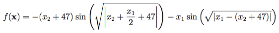
-512<xi<512
Global minimums f(x) = -959.6407 at (512, 404.2319)
| Number of iterations | Number of variables to optimize | Positions | Last function evaluation |
|---|---|---|---|
| 10 | 2 | -467.8004 381.2903 | -886.1135 |
| 50 | 2 | 511.2238 401.3568 | -951.5988 |
| 100 | 2 | 510.0009 401.2261 | -950.5605 |
4. Rastrigin function
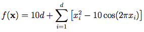
-5.12<xi<5.12
Global minimums f(x) = 0 at xi = 0 for i=0, 1, 2… n
| Number of iterations | Number of variables to optimize | Positions | Last function evaluation |
|---|---|---|---|
| 10 | 5 | 1.0387 -0.1816 1.0455 0.1107 -0.0802 | 12.3188 |
| 50 | 5 | 0.9958 -0.0004 -0.9954 0.9943 -0.9959 | 3.9803 |
| 100 | 5 | 0.9950 -0.9944 0.0000 -0.0000 0.0002 | 1.9900 |
| 1000 | 5 | 1.0e-04 *(-0.0511 0.1245 -0.3778 0.0225 0.5014) | 8.1888e-07 |
5. Griewank function

-600<xi<600
Global minimums f(x) = 0 at xi = 0 for i=0, 1, 2… n
| Number of iterations | Number of variables to optimize | Positions | Last function evaluation |
|---|---|---|---|
| 10 | 5 | 38.3575 -74.0117 -73.7770 -15.8375 -1.4636 | 4.1577 |
| 50 | 5 | -15.6588 9.0056 26.9700 18.9150 -35.2602 | 0.6801 |
| 100 | 5 | 15.6967 4.4584 -16.3073 -43.9101 14.0469 | 0.6652 |
| 1000 | 5 | 9.4132 13.3206 -5.4336 -0.0022 -21.0215 | 0.1847 |
| 10000 | 5 | -0.0004 -4.4383 5.4333 -6.2707 7.0076 | 0.0345 |
5. Experiments with FOA to minimize k-means algorithm for image clustering
For this experiments we use different sizes of images in pixels:
-
Icon: 10x10
-
Small: 128x128
-
Medium: 400x400
-
Large: 680x680
The experiments were made with the image’s original composition, its RGB values and without resizing the original photo.
The next parameters of the algorithm are fixed as follows:
-
Number of the iterations = 100
-
Number of clusters = 3
| Image size | RGB values per cluster | First k-means evaluation | Last k-means evaluation |
|---|---|---|---|
| Icon | [0, 0, 0], [251, 116, 49], [46, 176, 131] | 7,866.06 | 28.00 |
| Small | [0, 1, 0], [228, 230, 226], [121, 183, 37] | 1,586,918.28 | 1,025,600.00 |
| Medium | [116, 239, 255], [37, 240, 221], [255, 221, 0] | 8,744,951.20 | 4,007,400.00 |
| Large | [0, 0, 0], [248, 231, 156], [15, 66, 109] | 37,104,666.71 | 6,109,100.00 |
In this article we discuss an algorithm based on a nature process of trees survival, this algorithm is the Forest Optimization Algorithm (FOA). This algorithm is inspired by some procedures in the forest, specifically, the seed dispersal procedure. This procedure consist basically that in the forest, the trees with with most sunlight and better growth conditions will live longer that other trees and they use different methods to ensure future generations for many years. When seedling begins, some seeds fall right under their parent tree while others tend to travel long distances in search of better growing conditions and less competition. When they fall below their parent tree it is called local seed dispersal and when seeds travel long distances it is called long-distance seed dispersal. Seeds that travel long distance have better chances to survive and to become a tree because most of the seeds will fall under their parent tree, limiting resources and having a heavy competition for sunlight. In this article we used this algorithm to optimize the k-means objective function and then do color-based image segmentation with the results of the optimization of the objective function.
Ghaemi, M., & Feizi-Derakhshi, M. R. Forest Optimization Algorithm. Expert System with Applications (2014), http://dx.doi.org/10.1016/j.eswa.2014.05.009
Binu, D. Cluster analysis using optimization algorithms with newly designed objective functions. Expert Systems with Applications (2015), http://dx.doi.org/10.1016/j.eswa.2015.03.031
Cuevas, E., Oliva Navarro, D., Díaz Cortés, M. and Osuna Enciso, J. (2016). OPTIMIZACIÓN Algoritmos Programados con MATLAB. Alfaomega.
Surjanovic, S. & Bingham, D. (2013). Virtual Library of Simulation Experiments: Test Functions and Datasets. Retrieved from http://www.sfu.ca/\~ssurjano.