dbnlearn - Dynamic Bayesian Network Structure Learning, Parameter Learning and Forecasting

It allows to learn the structure of univariate time series, learning parameters and forecasting. Implements a model of Dynamic Bayesian Networks with temporal windows, with collections of linear regressors for Gaussian nodes, based on the introductory texts of Korb and Nicholson (2010) <doi:10.1201/b10391> and Nagarajan, Scutari and Lèbre (2013) <doi:10.1007/978-1-4614-6446-4>.

You can install the stable version of dbnlearn from CRAN:

install.packages("dbnlearn")

dbnlearn is available for developers, install from GitHub.

install.packages("devtools")
devtools::install_github("robson-fernandes/dbnlearn")

How to Use - Example applied to Amazon stock prediction

Data Reading

In this code snippet you get the opening prices of Amazon's stock in the period from 2015 to 2020. The data are obtained by the Yahoo Finance API.

library(quantmod)
library(dbnlearn)
library(bnviewer)
library(ggplot2)
library(MLmetrics)

amz <- getSymbols("AMZN", src = "yahoo", from = "2015-01-01", to = "2020-07-01", auto.assign = FALSE)

#Amazon Stock Time Series
ts <- amz$AMZN.Open

Pre-Processing and Data Separation

Then, the pre-processing step is performed which transforms the data considering a time window with time (t-n), where n is the number of steps passed. In this example, a time window of 30 was adopted.

The dataset is separated into 30% testing and 70% for model training.

#Time Series Preprocessing with time window = 30
X.ts = dbn.preprocessing(ts, window = 30)

#Define 70% Train and 30% Test Data Set
percent = 0.7
n = nrow(X.ts)

trainIndex <- seq_len(length.out = floor(x = percent * n))
X.ts.train <- X.ts[trainIndex,]
X.ts.test <- X.ts[-trainIndex,]

Learning the Structure of the Dynamic Bayesian Network and Visualization

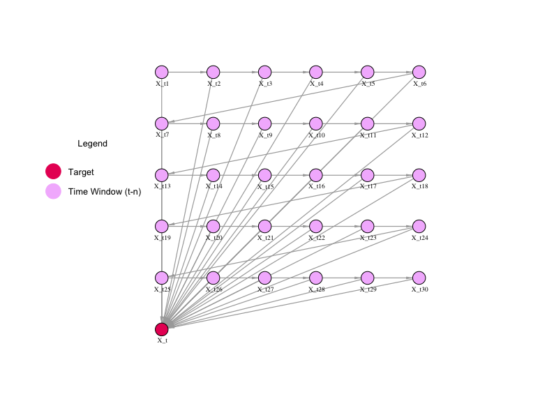
The 'dbn.learn' function is applied to learn the network structure based on the training samples, and then, the network is visualized by the 'viewer' function of the bnviewer package.

#Dynamic Bayesian Network Structure Learning
ts.learning = dbn.learn(X.ts.train)

#Visualization
viewer(ts.learning,
       bayesianNetwork.width = "100%",
       bayesianNetwork.height = "100vh",
       bayesianNetwork.enabled.interactive.mode = TRUE,
       edges.smooth = FALSE,
       bayesianNetwork.layout = "layout_with_gem",
       node.colors = list(background = "#f4bafd",
                          border = "#2b7ce9",
                          highlight = list(background = "#97c2fc",
                                           border = "#2b7ce9")),
       
       clusters.legend.title = list(text = "Legend"),
       
       clusters.legend.options = list(
         
         list(label = "Target (t)",
              shape = "icon",
              icon = list(code = "f111", size = 50, color = "#e91e63")),
         
         list(label = "Time Window (t-n)",
              shape = "icon",
              icon = list(code = "f111", size = 50, color = "#f4bafd"))
       ),
       
       clusters = list(
         list(label = "Target",
              shape = "icon",
              icon = list(code = "f111", color = "#e91e63"),
              nodes = list("X_t")),
         list(label = "Time Window (t-n)",
              shape = "icon",
              icon = list(code = "f111", color = "#f4bafd"),
              nodes = list("X_t1"))
       )
       
)

Visualization of the Dynamic Bayesian Network

Parameter Learning

Once having the network structure, parameter learning is performed using the maximum likelihood estimator.

#Dynamic Bayesian Network Fit
ts.fit = dbn.fit(ts.learning, X.ts.train)

Prediction

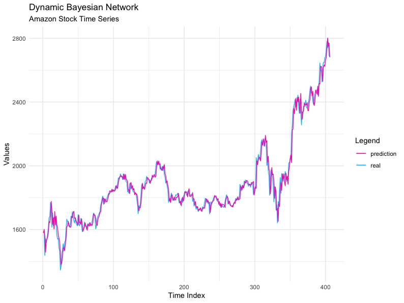
Now we can perform the data prediction considering the adjusted network, and validating with the test data.

#Predict values
prediction = dbn.predict(ts.fit, X.ts.test)

#Plot Real vs Predict
real = X.ts.test[, "X_t"]

df.validation = data.frame(list(real = real, prediction = prediction))

ggplot(df.validation, aes(seq(1:nrow(df.validation)))) +
  geom_line(aes(y = real, colour="real")) +
  geom_line(aes(y = prediction, colour="prediction")) +
  scale_color_manual(values = c(
    'real' = 'deepskyblue',
    'prediction' = 'maroon1')) +
  labs(title = "Dynamic Bayesian Network",
       subtitle = "Amazon Stock Time Series",
       colour = "Legend",
       x = "Time Index",
       y = "Values") + theme_minimal()

Viewing Actual Data and Prediction

It is possible to observe that the dynamic Bayesian network generated by the "dbnlearn" package, obtained an excellent performance, considering the millimeter adjustment between the test data versus the predicted data.

Evaluation Metrics

For evaluation, the MAPE metric (Mean Absolute Percentage Error) will be considered.

MAPE(prediction, real)

As an output we had a MAPE of 0,01578516. Excellent result!

hfshr/dbnlearn