The initial responses from other students explained that the file is a fixed length file that should be read with read.fwf(), and referred him to the 2000 ACS PUMS codebook for additional information on how to read the file.
Pointing the student to the codebook was not sufficient for him to solve the problem on his own. Since the problem was an interesting "real world" application of the material covered in Getting and Cleaning Data, we developed the solution that is stored within this Github repository.
The lgreski/acsexample repository includes three files that can be used to read the data from a single state's contribution to the 2000 American Community Survey Public Use Microdata Sample. The American Community Survey includes extensive documentation, ranging from code books to user notes and errata. A complete inventory of all available PUMS data is also available on the U.S. Census Bureau website. Additional files in the repository include the README.md and images that are referenced within the README.
| File Name | Description |
|---|---|
| README.md | Documentation explaining the project and how to use files contained in the repository. |
| read PUMS codebook.R | R script to read the American Community Survey Public Use Microdata Sample codebook and a single state's data. The codebook is distributed as a Microsoft Excel spreadsheet. The ACS survey data read is the output from the split PUMS person and households.R script. The script uses read.fwf() to read the survey data. |
| read PUMS codebook - readr version.R | R script to read the American Community Survey Public Use Microdata Sample codebook and a single state's data. The codebook is distributed as a Microsoft Excel spreadsheet. The ACS survey data read is the output from the split PUMS person and households.R script. The script uses Hadley Wickham's readr package read_fwf() function to read the survey data. |
| split PUMS person and households.R | R script to parse the census file and separate into two files for downstream processing: a person-level file and a household-level file. The script uses readLines() and substr() to split the data into the appropriate output files. |
| *.png | Graphics images to be embedded in the README.md file |
| data/5%_PUMS_record_layout.xls | Local copy of codebook describing the PUMS data file layout. |
Techniques for reading data from a variety of sources are covered during weeks one and two, including XML, JSON, Excel files, application APIs, and other sources.
One of the key challenges faced by students in the Johns Hopkins Data Science Specialization is how to generalize the teaching of a specific technique to make it usable to solve problems beyond the specific example(s) demonstrated in the lectures.
To solve this particular problem, we needed to combine multiple techniques that we had learned in the class, in a manner that would not be obvious to many students enrolled in the class.
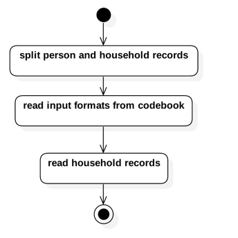
As a learning exercise, the solution posted for reading the PUMS data is noteworthy because it combines three techniques into an elegant solution for reading this data in R, including:
- Use of
readLines()to split the data into household and person level records, - Use of
read.xlsx()to generate the content required as arguments toread.fwf(), and - Use of
readr::read_fwf()instead ofread.fwf()to reduce the data load time from 19 minutes to 9 seconds on a laptop with an Intel i5 processor.
Our task here is to read the PUMS data for the state of New York, which was ranked #3 in population as of the 2000 Census, with just under 18 million in population. As expected the PUMS data file is relatively large: 411.9 Mb.
To complete our task, we need to understand the structure of the input data file. Fortunately, there is plenty of documentation about the 2000 PUMS data, thanks to the U.S. Census Bureau (and U.S. taxpayers). In addition to a 724 page user guide, data layouts and value labels for the 5% sample are explained in a series of Excel spreadsheets stored along with the state by state data.
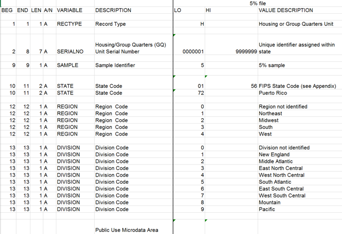
The 5% sample code book spreadsheet contains two worksheets: Housing and Person. The Housing Units tab explains variables by column number in the left part of the worksheet, and provides value labels for the categorical variables (factors) that are in the survey, as illustrated below.
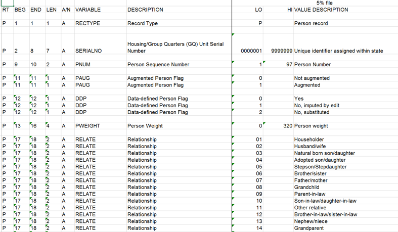
The Person worksheet includes the same information for person records.
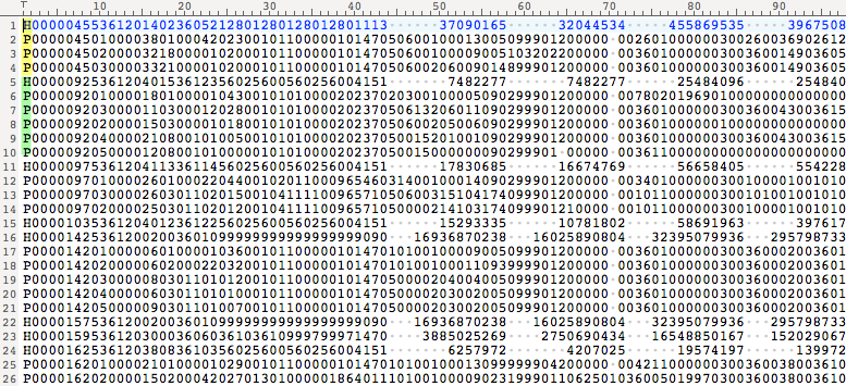
When we look at the raw data file for person records, we find that there is not a predictable relationship between housing records and person records in the data file (i.e. 1 housing unit, then 3 person units, then 1 housing unit, and so on). The key that associates the two record types is SERIALNO -- the Housing / Group Quarters (GQ) Unit Serial Number. The following snapshot from the raw data illustrates the problem, as the first household is associated with 3 person records, and the second household is associated with 5 person records.
Therefore, the easiest way to split the file is to use readLines() to read the entire file as a set of character strings, and then, record by record, check the first character to see whether it is P or H.
If one is familiar with record-oriented data processing models, separating the data with R is very straightforward.
First, we initialize three files: the input file and two output files, one for persons and one for households Then we read the data file into memory with readLines(), and using lapply(), write each row to either a person or household output file based on the character in column one.
The code to evaluate each row and write it to the correct file is implemented as an anonymous function.
inFile <- "./data/REVISEDPUMS5_36.TXT"
outputPersonFile <- "./data/PUMS_person_NY.txt"
outputHouseholdFile <- "./data/PUMS_household_NY.txt"

theInput <- readLines(inFile,n = -1)
theResult <- lapply(theInput,function(x) {
 if(substr(x,1,1)=="P") {cat(x,file=outputPersonFile,sep="\n",append=TRUE)}
 else {cat(x,file=outputHouseholdFile,sep="\n",append=TRUE)}
})
On a laptop with an Intel i5 processor, 8 Gb of RAM, and a 512 Gb solid state disk, we are able to split the data into the required output files in about one minute. While it is technically possible to write a program that reads the data row by row, initializes a row for a data frame, then builds the data frame with rbind(), the benefit of the file-based approach is its simplicity. Additionally, due to the way that rbind() allocates memory, it would perform significantly worse than using readLines().
Having split the file into person and household records, we can use existing R functions to load the data, rather than building a custom parser to load the data into a data frame.
Taking another look at the code book spreadsheet, the tab for the person-level data has 1,219 rows. Manually creating the length vector for all these variables as required by the read.fwf() function would be tedious to create, and difficult to debug.
Here is where knowing the best way to do something in R is invaluable. The spreadsheet itself can be used to generate the input length vector AND column names for the resulting data frame, not only saving a lot of tedious work, but also ensuring accuracy of the input arguments to read.fwf().
On closer inspection, we notice that many of the rows in the left part of the worksheet are duplicates because there is a set of columns in the middle of the spreadsheet that provide variable labels for each variable to its left.
Therefore, we can read columns 1 - 7 with read.xlsx() and use the data.table::unique() function to eliminate the duplicates.
Also, to improve readability of the spreadsheet, the authors included a number of empty rows. A simple !is.na(codeBook$LEN) on the column length variable can remove the blank row, bringing us to a total of 174 variables in the person file. The R code required to process the code book is listed below.
library(xlsx)
# using vgrep() determine the row and column indexes
# note that column names are in row 2
# reference: http://www.jargon.net/jargonfile/v/vgrep.html
colIndex <- 1:7
rowIndex <- 2:1219
codeBook <- read.xlsx("./data/5pct_PUMS_record_layout.xls",
                      sheetIndex=2,
                      colIndex=colIndex,
                      rowIndex=rowIndex,
                      stringsAsFactors=FALSE)
# remove blank rows
codeBook <- codeBook[!is.na(codeBook$VARIABLE),]
# remove duplicate rows
library(data.table)
codeBook <- unique(as.data.table(codeBook))

# remove NA rows by setting length to a numeric variable, and processing
# with !is.na
codeBook$LEN <- as.numeric(codeBook$LEN)
codeBook <- codeBook[!is.na(codeBook$LEN)]
The LEN and VARIABLE columns in the code book are exactly what we need to specify in read.fwf() to avoid a lot of tedious manual effort building the vectors required for the widths and col.names arguments.
For pedagogical purposes we explicitly created vectors for these arguments, but we could have referenced the vectors directly from the codeBook data frame. To reduce the memory allocation overhead in read.fwf(), we set the n= argument to 953076, the number of rows in the input file. The code to load the PUMS data into a data frame is as follows.
# set widths vector to LEN (length) column
colWidths <- codeBook$LEN

# set column names to the VARIABLE column in codebook
colNames <- codeBook$VARIABLE
# read PUMS data previously separated by split PUMS R script
personData <- read.fwf("./data/PUMS_person_NY.txt",
                       colWidths,
                       header=FALSE,
                       n=953076,
                       col.names = colNames,
                       stringsAsFactors=FALSE)
The R code required to process the spreadsheet and create a data frame required only 11 statements, including two library() calls. Our laptop was able to read the 950K records and create a data frame in R in about 19.6 minutes. The resulting R data frame consumed 701.8Mb of memory. After posting this solution on the course Discussion Forum, David Hood (a Community Mentor) wrote that earlier in 2015, Hadley Wickham had published an R package to dramatically speed the reading of data into R.
We then replaced read.fwf() with readr::read_fwf() and reduced the load time from 19 minutes to 8.98 seconds. Additionally, the size of the data frame dropped from 701.8Mb to 341.2Mb, a greater than 50% reduction in memory use.
Code for the readr::read_fwf() solution is included below.
# use Wickham's readr package to read the data
library(readr)
personData <- read_fwf("./data/PUMS_person_NY.txt",
                       fwf_widths(colWidths, col_names=colNames),
                       n_max=953076)
readr::read_fwf() for the base read.fwf() it also becomes a high performance solution.


