hoangthangta/FCN-KAN

Kolmogorov–Arnold Networks with modified activation (using fully connected network to represent the activation)

FCN-KAN

Kolmogorov–Arnold Networks with modified activation (using FCN + positional encoding to represent the activation). The code utilizes torch.vmap to accelerate and simplify the process.

Experiment

Running the following code for quick experiment:

python experiment.py

Example usage

from kan_layer import KANLayer

model = nn.Sequential(
        KANLayer(2, 5),
        KANLayer(5, 1)
    )

x = torch.randn(16, 2)
y = model(x)
# y.shape = (16, 1)

Visualization

I experimented with a simple objective function:

$$f(x,y)=\exp(\sin(\pi x) + y^2)$$

def target_fn(input):
    # f(x,y)=exp(sin(pi * x) + y^2)
    if len(input.shape) == 1:
        x, y = input
    else:
        x, y = input[:, 0], input[:, 1]
    return torch.exp(torch.sin(torch.pi * x) + y**2)

The first experiment set the network as:

dims = [2, 5, 1]
model = nn.Sequential(
    KANLayer(dims[0], dims[1]),
    KANLayer(dims[1], dims[2])
)

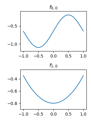
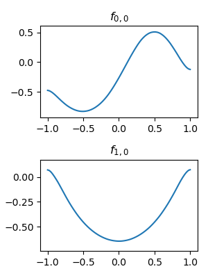
After training on this, the activation function did learn the $\sin(\pi x)$ and $x^2$ functions:

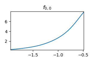
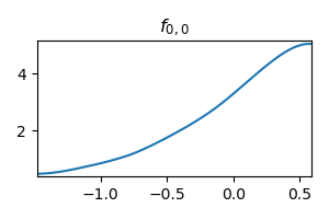
The exponential function is also been learned for the second layer:

For better interpretability, we can set the network as:

dims = [2, 1, 1]
model = nn.Sequential(
    KANLayer(dims[0], dims[1]),
    KANLayer(dims[1], dims[2])
)

Both the first layer and the second layer learning exactly the target function:

Second layer learning the exponential function:

Linear Interpolation Version

from kan_layer import KANInterpoLayer

model = nn.Sequential(
        KANInterpoLayer(2, 5),
        KANInterpoLayer(5, 1)
    )

x = torch.randn(16, 2)
y = model(x)
# y.shape = (16, 1)

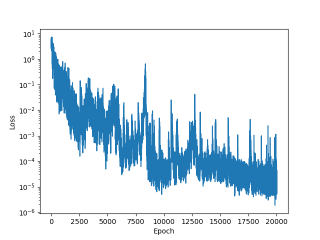
The result shows similar performance. However, this version is harder to train. I guess it is because each parameter only affect the behavior locally, making it harder to cross local minima, or zero-gradient points. Adding smooth_penalty may help.