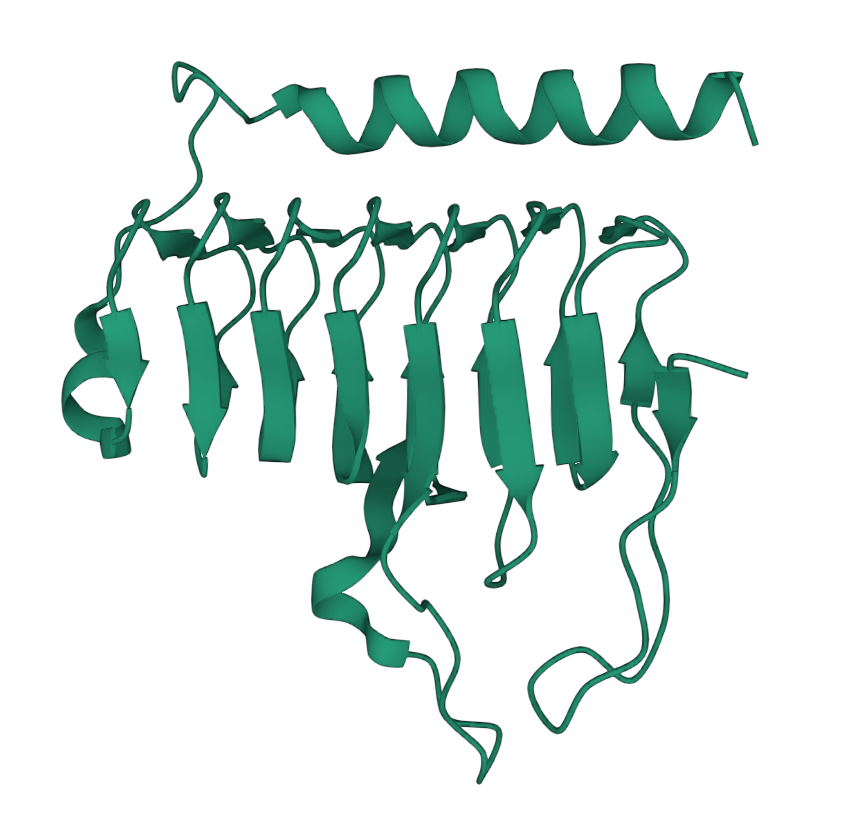
faltwerk: A Jupyter Notebook repository from hoelzer

Faltwerk

faltwerk is a library for spatial exploratory data analysis of protein structures. It helps parse them, select items of interest, generate and visualise various protein annotations, and then provide convenient interfaces for downstream tools to perform e. g. as spatial regression. The most convenient way to run faltwerk is in a jupyter notebook.

Why this library? Exploratory analysis of protein structures in a REPL such as jupyter notebooks and outside of point-and-click tools can be surprisingly annoying.

By "exploratory", we mean spatial. The curious thing about proteins is that by design they are a linear string of residues, but then folds up into the functionally active structure. Nature selects on the 3D structure, but we typically analyse the linear sequence (DNA sequencing). foldspace really wants to bridge this gap. More specifically, here are some use cases:

Annotate solvent access, active centers and more
Some regions in the amino acid sequence are more conserved than others across species. Which regions in the 3D structure do they correspond to?
Are there any significant spatial hotspots where residues experience positive selection?
Do observed mutations cluster in any part of the protein, for example in regions that interface other proteins (protein binding sites) or active sites of the protein?
A hotspot/ cluster has been identified; which protein features if any can explain this occurance. For example, is the cluster associated with known protein-binding sites?
What's the spatial relationship between mutations deemed pathogenic and the annotated functional domains of a protein?

PRs and suggestions welcome! The awesome Anvio has a structure module, should you be dissatisfied with faltwerk.

Install

chmod +x install.sh
./install.sh
# ... or just follow the steps therein manually

# Get Pfam database (Version v31 -- this matters!)
wget http://ftp.ebi.ac.uk/pub/databases/Pfam/releases/Pfam31.0/Pfam-A.hmm.dat.gz
wget http://ftp.ebi.ac.uk/pub/databases/Pfam/releases/Pfam31.0/Pfam-A.hmm.gz
gunzip *
hmmpress Pfam-A.hmm

Usage

We assume that all protein structures contain a single, and if you are not analysing protein complexes, then you want the structures to only contain a single chain, also. A simple way to clean a query pdb file is through pdb-tools (http://www.bonvinlab.org/pdb-tools/). AlphaFold2 predictions as generated by ColabFold are ideal.

To get an overview of what you can do with faltwerk and to interact with the data and code, we provide a notebook:

jupyter notebook example.ipynb

To give an idea of what it looks like to use faltwerk:

# Load data
from faltwerk.models import Fold, AlphaFold
# ... (for details see notebook)

fp = 'data/alphafold2/transferrin/test_08df6_unrelaxed_rank_1_model_3.pdb'
model = Fold(fp)

# or
fp = 'data/alphafold2/transferrin/'
af = AlphaFold(fp)
model = af.best

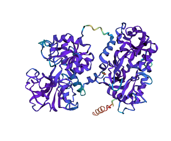
# Visualise pLDDT (how good is AF2 the prediction)
ly = Layout(model).geom_ribbon('plddt', palette='rainbow_r')

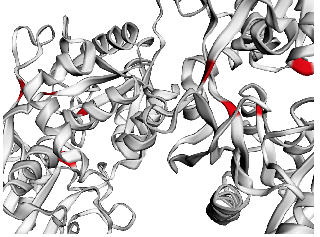
# Predict ligand binding sites using the "InteracDome" approach
b = Binding(model, 'representable')
b.predict_binding_(pfam)
binding = b.get_binding('PF00405.16', 'FE')
fe = [i for i, j in enumerate(binding) if j > .5]

ly = Layout(model)
# select
fe_ = ly.select(residues=fe)
# style
ly.geom_ribbon(color='#ffffff')
ly.geom_ribbon(selection=fe_, color='red')
ly.render().show()

# Test for spatial signal in residues that are e. g. mutated or under positive
# natural selection. Here we use residues from Barber et al., Science, 2014
# (https://www.science.org/doi/10.1126/science.1259329) that are under positive
# selection.
original = [153, 253, 382, 434, 435, 436, 439, 558, 574, 575, 576, 591, 592, 593, 614, 617, 619, 625]

# -1 bc/ positions from manuscript are 1-based 
barber2014 = [i-1 for i in original]
selection = [1 if i in barber2014 else 0 for i in range(len(model))]

# (1) Spatial autocorrelation, i. e. "hotspots" in selected features, here using
# the Getis-Ord metric.
FDR = 0.05
hotspots = find_hotspots(
    model,
    selection,
    method='getis_ord',
    angstrom=8,
    false_discovery_rate=FDR,
    test_two_sided=False)

# (2) Point density analysis, here using HDBSCAN.
clusters = cluster(model, hotspots, min_cluster_size=5)

# Annotate model
model.annotate_many_({
    'selection': selection,
    'hotspots': hotspots,
    'clusters': clusters})

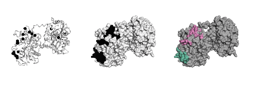
# Build figure like a layer cake
ly = Layout(model, panel_size=(200, 200), grid=(1, 3), linked=True)

pos = ly.select(residues=barber2014, elements=['CA'], chain='A')

ly.geom_ribbon(color='#ffffff')
ly.geom_sphere(selection=pos, color='black')
ly.geom_surface('hotspots', palette='binary', panel=(0, 1))
ly.geom_surface('clusters', palette='Set2_r', panel=(0, 2))
ly.render().show()

From here, faltwerk allows to easily interact with downstream tools like altair for visualisation of features or pysal for spatial regression (see notebook example.ipynb)

df = pd.DataFrame.from_dict(
    flatten(model.annotation, expected_track_length=len(model)))

hoelzer/faltwerk

Faltwerk

Install

Usage