hrbigelow/draw

Deep Recurrent Attentive Writer

Tensorflow v2.6 implementation of the Deep Recurrent Attentive Writer

This is a TF v2.6 implementation of the Deep Recurrent Attentive Writer from https://arxiv.org/pdf/1502.04623.pdf. It is based on Eric Jang's implementation here, but written in TF v2.6, and upgraded to allow training on CIFAR10 color images.

Usage

python draw.py --help

# MNIST training
python draw.py --hps='mnist' --data_dir=/path/to/data/tmp \
   --ckpt_template=/path/to/ckpt/run3.%.ckpt \
   --tboard_logdir=/path/to/tb/log/run3/

# CIFAR10 training
python draw.py --hps='cifar' --data_dir=/path/to/data/tmp \
   --ckpt_template=/path/to/ckpt/run3.%.ckpt \
   --tboard_logdir=/path/to/tb/log/run3/

To generate new data using a trained model, use the weights file included in this repo:

# nrow * ncol must equal batch_size
python gen_data.py --hps='mnist' --ckpt_path=ckpt/run3.17500.ckpt \
    --img_path=/path/to/results/run3.17500 --nrow=10 --ncol=10

python gen_data.py --hps='cifar' --ckpt_path=ckpt/cifar.run2.9500.ckpt \
    --img_path=/path/to/results/cifar.run2 --nrow=10 --ncol=20

This will create a series of images "imagined" by the trained decoder model, one at each timestep during the iterative generation process. You can then make them into a gif with:

convert -delay 10 -loop 0 run3.17500_?.png run3.17500_??.png run3.17500.gif
animate run3.17500.gif

draw.py records the KL loss, "reconstruction loss", and the sum of the two in the tensorboard format. Unfortunately, tensorboard doesn't allow viewing them in one plot, but you can generate such a plot using the following:

# first sign in to https://tensorboard.dev
tensorboard dev upload --logdir TB_LOGDIR
python plot_tboard.py --exp_id=EXPERIMENT_ID --run=RUN_SUBDIR

# For example:
tensorboard dev upload --logdir /path/to/tb/log
python plot_tboard.py --exp_id=mgSAaxxyRkCQFnEzmMFaxA --run=run3
# save the displayed plot

Here is a result on the binarized MNIST data. The trained model is in ckpt/run3.17500.ckpt

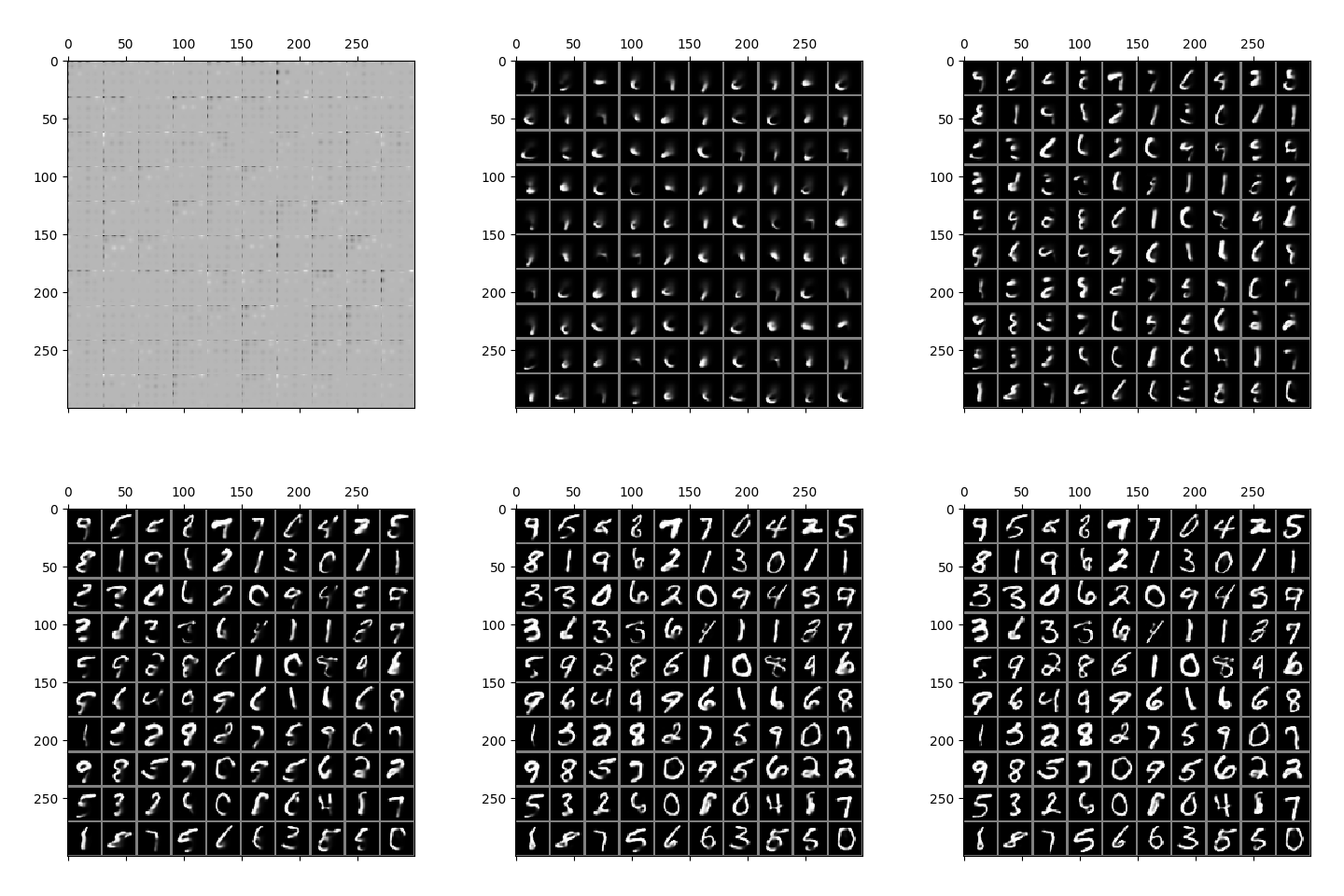
The animated MNIST gif shows 100 images sampled from the decoder, each timestep of the gif corresponding to one of the 64 timesteps during the decoder's progressive generation of the images. No actual MNIST digits are used in any part of this generation process, and the process does not use the encoder at all.

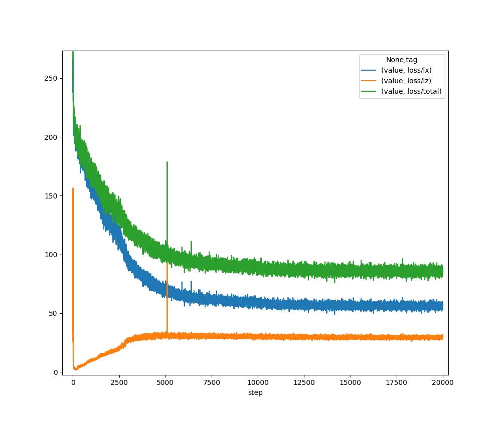
During training this model, one thing that is apparent is that the Lz loss term initially goes down at the beginning of training, but then starts to climb. The gain in Lz is more than compensated by a loss of Lx, resulting in the total loss going down. Loosely speaking, from an information theoretic point of view, the quantity Lz goes up as the mutual information I(X;Z) increases. This is appropriate as the encoder learns to convey enough information to the decoder in order to maximize log likelihood.

Here is a result on CIFAR10 data. The trained model is in ckpt/cifar.run2.9500.ckpt.

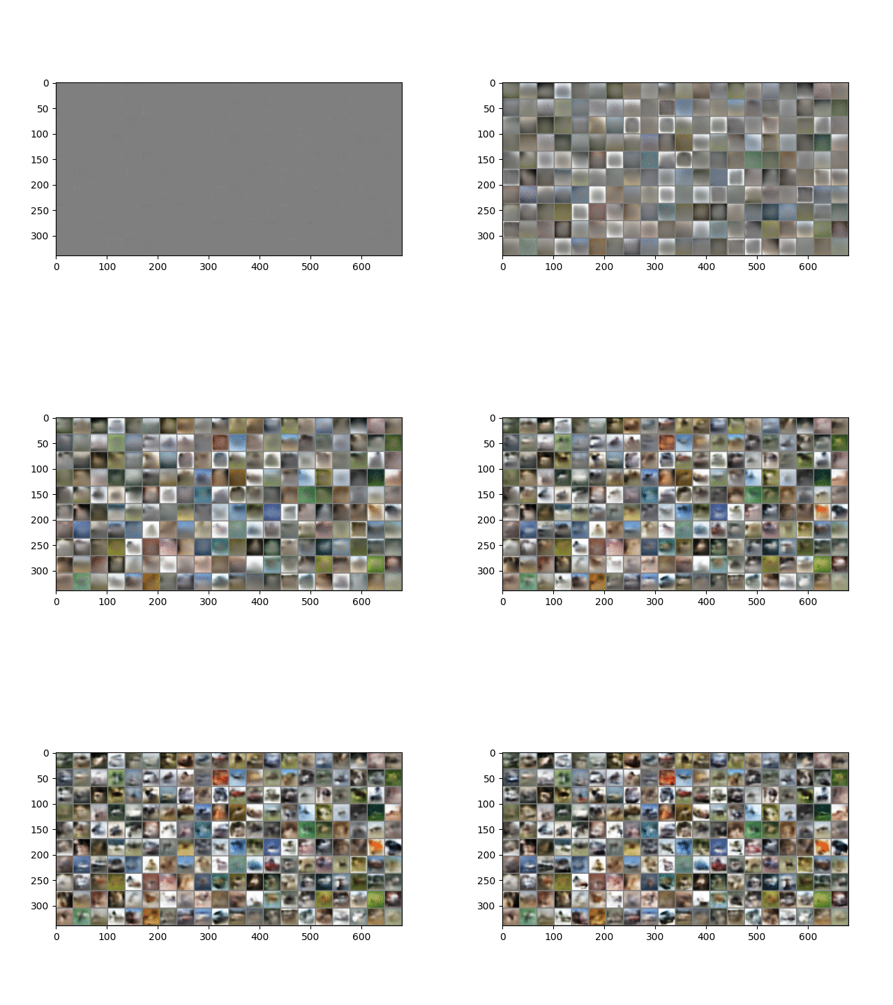
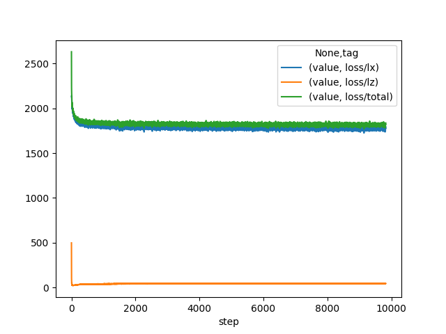
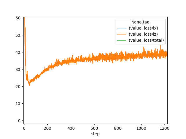
A similar phenomenon during training is observed here, except that the CIFAR images are 32 x 32 and 3 channels, and so represent more than 3x the information contained in MNIST images. As described in the paper, image generation is performed in the same way except that each channel of each pixel is a separate binomial sampling.

Discussion

Tensorboard runs are available here. In run1, the latent space "collapsed", and loss/lz went to zero. This was not repeatable for the next several trial training runs, even though they all used the same hyperparameters.

During training, the summed KL divergence, summed over the timesteps (equation 10 in the paper) noted L^z, starts out high, then quickly falls to a value around 2, and then slowly climbs. In the collapse incident, it fell to zero and remained there. In the successful runs, the slow climb indicates that the encoder is learning to transmit more information that is useful for the decoder to reconstruct the image.

One point to make is that equation 11 in the paper is a bit vague. A more complete derivation of KL divergence between two multivariate Gaussians is given here and in the last equation of Appendix B of Kingma and Welling's famous VAE paper. It is implemented in the code for a single timestep here. In my experiments, it was important to make sure that Lz and Lx are both averaged over the batch dimension.

One other point to make. The target images are binarized MNIST images, which means that each pixel value is assigned a value of 0 or 1 (on or off). In the context of this paper, each target pixel is interpreted as a binomial probability. Similarly, the decoder generates a binomial probability for each pixel (now varying continuously in [0, 1)). The final image is generated by independent binomial samples, one for each pixel.

The reconstruction loss L^x mentioned in equation 9 turns out to be KL divergence D(P||Q) = H(P, Q) - H(P) where P is the target distribution (with 0 or 1 as a probability for each pixel) and Q is the decoder distribution. This is because H(P) = 0, and H(P, Q) is just a sum over -log(Q) values corresponding to whichever binary outcome is given by the target image. The relevant code is here

I chose to use tf.nn.sigmoid_cross_entropy_with_logits since it provides cross-entropies for each pixel individually and allows summing later. There is a Keras binary cross entropy function as well, but it seems to average across the dimensions rather than sum, which is not what's needed here.

Another thing to note: There is a spike in lz at step 5099 in training run 3. This for some reason is not visible on tensorboard.dev, because that interface doesn't display every timestep. However, the data uploaded to it does include every timestep, and the code in plot_tboard.py downloads directly from tensorboard.dev. I'm not sure why it is not displayed, but it is a real blip.