Create Dorling Cartograms from Contiguous Region Shapefiles
Create Dorling Cartograms from Contiguous Region Shapefiles
dorling_from_sp: Compute center coordinates, circle radii and Dorling polygons from input polygons and values
The following functions are implemented:
devtools::install_github("hrbrmstr/spdorling")library(spdorling)
# current verison
packageVersion("spdorling")## [1] '0.1.0'
library(albersusa) # hrbrmstr/albersusa
library(hrbrthemes)
library(tidyverse)

usa <- albersusa::usa_composite(proj = "laea")
usa <- subset(usa, !(name %in% c("Alaska", "Hawaii", "District of Columbia")))

set.seed(2018)
usa$val <- sample(10000, 48)

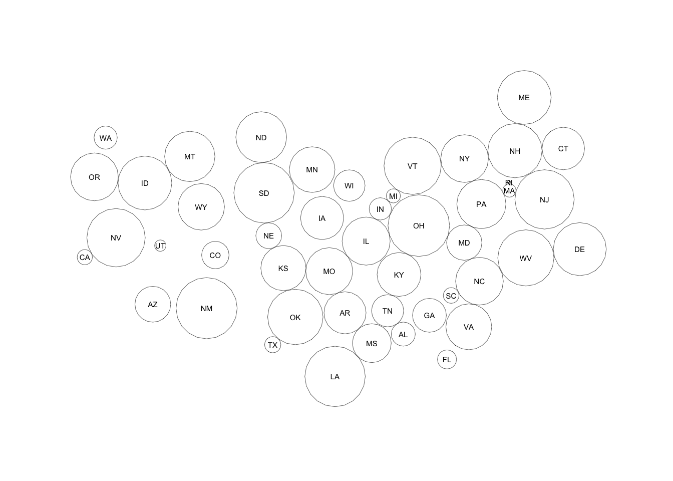
dor <- dorling_from_sp(usa, value=usa$val, quiet=FALSE)
## Scale factor of 1 => number of overlaps : 12
## Scale factor of 0.9795918 => number of overlaps : 15
## Scale factor of 0.9591837 => number of overlaps : 7
## Scale factor of 0.9387755 => number of overlaps : 9
## Scale factor of 0.9183673 => number of overlaps : 8
## Scale factor of 0.8979592 => number of overlaps : 6
## Scale factor of 0.877551 => number of overlaps : 0
discs_df <- fortify(dor$discs)

as_data_frame(dor$xy) %>%
  set_names(c("lng", "lat")) %>%
  mutate(iso2c = usa$iso_3166_2) -> usa_labs

ggplot() +
  geom_polygon(
    data = discs_df, aes(long, lat, group=group),
    size=0.125, color="#2b2b2b", fill="#00000000"
  ) +
  geom_text(data = usa_labs, aes(lng, lat, label=iso2c), size=2) +
  coord_fixed() +
  labs(x=NULL, y=NULL) +
  theme_ipsum_rc(grid="") +
theme(axis.text=element_blank())library(sp)
library(rgdal)## rgdal: version: 1.2-18, (SVN revision 718)
## Geospatial Data Abstraction Library extensions to R successfully loaded
## Loaded GDAL runtime: GDAL 2.1.3, released 2017/20/01
## Path to GDAL shared files: /Library/Frameworks/R.framework/Versions/3.5/Resources/library/rgdal/gdal
## GDAL binary built with GEOS: FALSE
## Loaded PROJ.4 runtime: Rel. 4.9.3, 15 August 2016, [PJ_VERSION: 493]
## Path to PROJ.4 shared files: /Library/Frameworks/R.framework/Versions/3.5/Resources/library/rgdal/proj
## Linking to sp version: 1.2-7
readOGR(
  system.file("extdat", "swiss-cantons.json", package="spdorling"),
  verbose = FALSE,
  stringsAsFactors = FALSE
) -> cantons

# convert it to equal area
SpatialPolygonsDataFrame(
  spTransform(cantons, CRS("+proj=aea +lat_1=45.96 +lat_2=47.50 +lon_0=8.34")),
  data = cantons@data
) -> cantons

set.seed(2018)
cantons$val <- sample(10000, nrow(cantons@data))

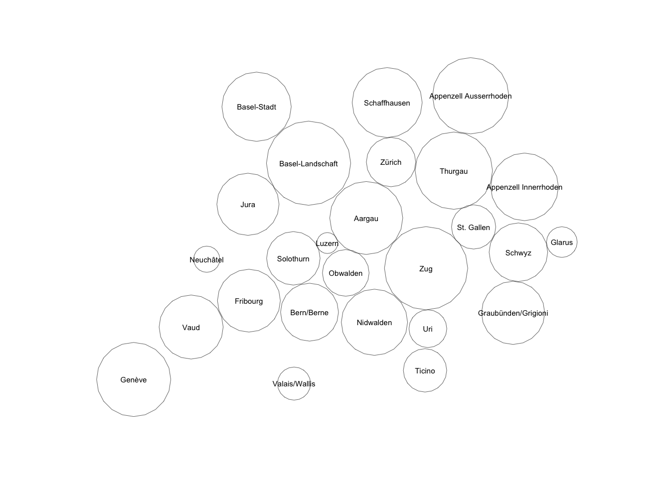
dor <- dorling_from_sp(cantons, value=cantons$val, quiet=FALSE)
## Scale factor of 1 => number of overlaps : 17
## Scale factor of 0.9795918 => number of overlaps : 5
## Scale factor of 0.9591837 => number of overlaps : 9
## Scale factor of 0.9387755 => number of overlaps : 7
## Scale factor of 0.9183673 => number of overlaps : 15
## Scale factor of 0.8979592 => number of overlaps : 7
## Scale factor of 0.877551 => number of overlaps : 8
## Scale factor of 0.8571429 => number of overlaps : 0
discs_df <- fortify(dor$discs)

as_data_frame(dor$xy) %>%
  set_names(c("lng", "lat")) %>%
  mutate(name = cantons$name) -> cantons_labs

ggplot() +
  geom_polygon(
    data = discs_df, aes(long, lat, group=group),
    size=0.125, color="#2b2b2b", fill="#00000000"
  ) +
  geom_text(data = cantons_labs, aes(lng, lat, label=name), size=2) +
  coord_fixed() +
  labs(x=NULL, y=NULL) +
  theme_ipsum_rc(grid="") +
  theme(axis.text=element_blank())
