Read, Inspect, Manipulate, and Save (ASE) Color Swatch Files (ACO/ASE/GPL/SOC/KDE/COLORS)
In Envisioning Information, Edward Tufte says “…avoiding catastrophe
becomes the first principle in bringing color to information: Above all,
do no harm.” R users gain a quick upper hand in adhering to this “do no
harm” thanks to sane defaults in ggplot2 and packages like viridis,
ggthemes or RColorBrewer that enable use of established and good
color palettes.
If you do visualization work in conjunction with a design shop or organization that establishes their own palettes and themes there will often be standard palettes that must be adhered to. These are usually stored and shared in some type of Adobe swatch file format. There are also many sites like Adobe Color CC and COLOUR Lovers where folks can create and share color palettes. Plus, there are thousands of other palette files in dozens of palette formates.
This package enables you to use the colors straight from .ase, .aso,
.gpl, .soc or .color files and avoid the cutting/pasting of hex
codes or using color pickers to extract the color information. You can
read these swatch files directly from the internet and/or include the
files directly in your R projects. This will make it easier to modify a
resource versus change code.
NOTE that just beacuse an ASE, ACO, GPL, SOC or color file exists on the internet does not mean that it will let you “do no harm”. You still need to use good judgement from knowledge/experience (or advice from experts) to ensure you are using colors effectively. This package just opens up the world of colors in R a little bit more.
The following functions are implemented:
read_palette: Generic function to read any supported palette type (determined by extension)read_aco: Read colors from Adobe Color (ACO) filesread_ase: Read colors from Adobe Swatch Exchange (ASE) filesread_gpl: Read GIMP Palette (GPL) filesread_soc: Read OpenOffice palette (SOC) filesread_kde: Read KDE Palette (colors) filesshow_palette: Display a color paletteadd_color: Add a named color to an ASE swatch objectase_encode: Encode a built ASE object for outputcreate_ase: Create an ASE objecthex_to_ase: Convert a list of named, hexadecimal RBG colors into an ASE object
- ACO/ASE Grayscale support (just need to find or gen Grayscale ASE/ACO files, if you have a few please hook me up)
- ACO/ASE LAB support (could use some help with this)
- Writing out palette files (somewhat done!)
devtools::install_github("hrbrmstr/swatches")library(swatches)
# current verison
packageVersion("swatches")## [1] '0.6.0'
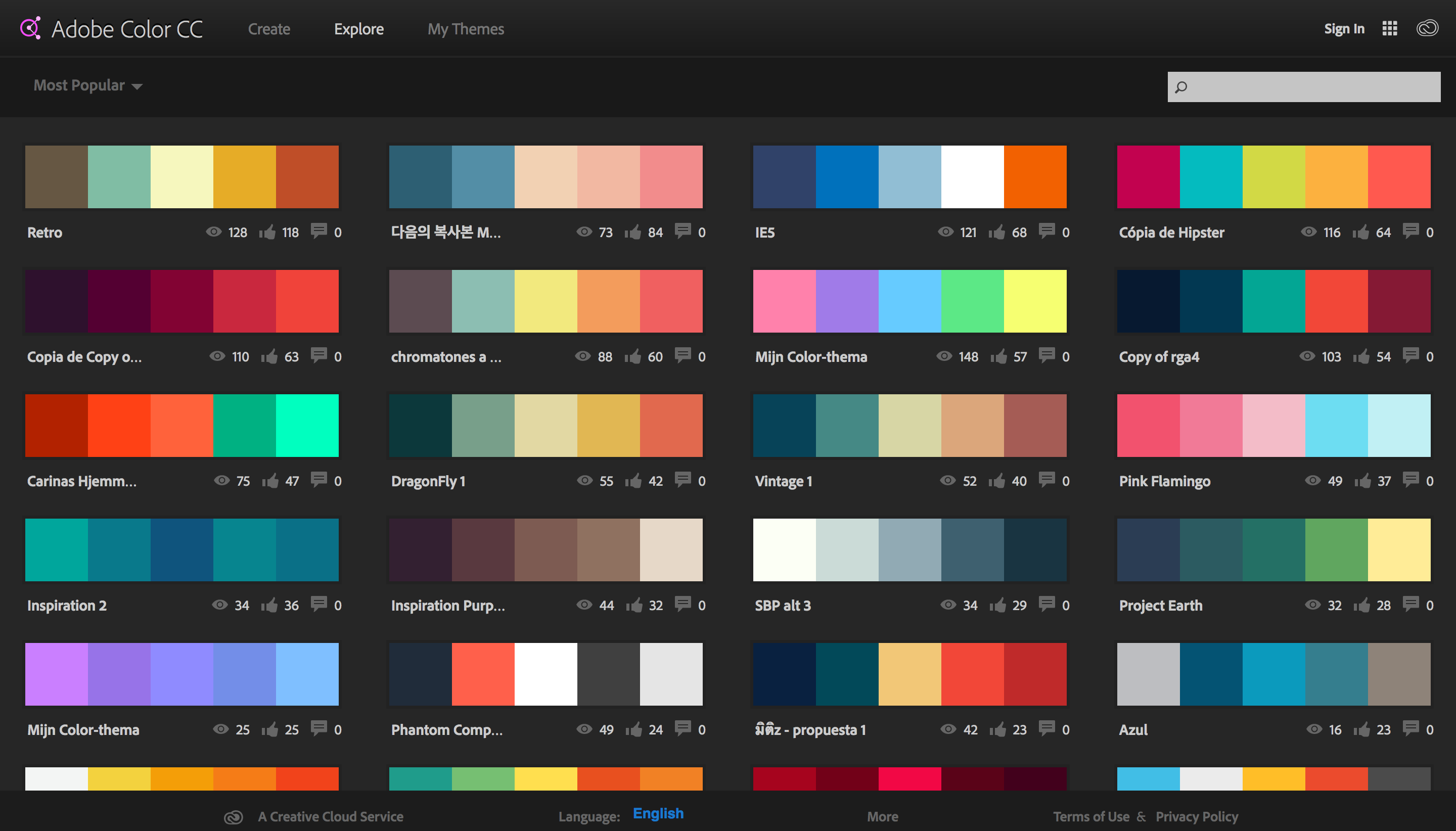
One good source for palettes is the “Most Popular” section on Adobe Color CC. If you use the Adobe ecosystem, you can sync ASE palette files directly locally or download them directly (registration required).
The “Herbs and Spice” and “Keep the Change” palettes are kinda nifty, and also included in this package (since Adobe has yet to release the new API for the color site for automatic downloading). We can take a quick look at both of them. Here they are from the web site:
And, there they are via this package:
herbs_and_spice <- read_ase(system.file("palettes", "herbs_and_spice.ase", package="swatches"))
print(herbs_and_spice)
##
## "#5A1F00" "#D1570D" "#FDE792" "#477725" "#A9CC66"
show_palette(herbs_and_spice)keep_the_change <- read_ase(system.file("palettes", "keep_the_change.ase", package="swatches"))
print(keep_the_change)##
## "#6B0C22" "#D9042B" "#F4CB89" "#588C8C" "#011C26"
show_palette(keep_the_change)As said earlier, you can also read directly from a URL. Here is a “metal” palette ripped straight from github:
metal <- read_ase("https://github.com/picwellwisher12pk/en_us/raw/master/Swatches/Metal.ase")
print(metal)
## C=0 M=0 Y=30 K=0 C=2 M=20 Y=94 K=0 C=0 M=6 Y=47 K=0
## "#ffffb3" "#fbcc0f" "#feef89"
## C=20 M=40 Y=96 K=7 C=16 M=32 Y=82 K=5 C=4 M=14 Y=60 K=8
## "#bf9009" "#cba62c" "#e2cc5e"
## C=1 M=19 Y=90 K=0 C=0 M=5 Y=42 K=5 C=8 M=4 Y=3 K=27
## "#fccf1b" "#f2e78c" "#acb3b5"
## C=17 M=8 Y=5 K=39 C=2 M=0 Y=4 K=16 C=6 M=7 Y=4 K=22
## "#829094" "#d2d7ce" "#bdbbc1"
## C=11 M=13 Y=8 K=38 C=8 M=9 Y=6 K=28 C=3 M=4 Y=3 K=14
## "#8d8a91" "#a9a7ad" "#d3d2d5"
## C=1 M=1 Y=1 K=7 C=4 M=3 Y=3 K=7 C=18 M=8 Y=10 K=48
## "#ececed" "#e3e6e6" "#6e7c79"
## C=10 M=5 Y=6 K=24 C=17 M=11 Y=13 K=0 C=31 M=24 Y=25 K=0
## "#b0b9b7" "#d5e3de" "#b0c4c0"
## C=64 M=47 Y=52 K=19 C=51 M=37 Y=40 K=4 C=71 M=53 Y=57 K=32
## "#4a6e64" "#7a9c94" "#33524b"
## C=0 M=7 Y=24 K=5 C=18 M=43 Y=89 K=7 C=1 M=12 Y=50 K=6 1
## "#f3e3bb" "#c4871b" "#edd378"
## C=21 M=49 Y=100 K=7 C=16 M=38 Y=79 K=6 C=0 M=19 Y=54 K=8
## "#bd7a00" "#ca9434" "#ebbf6c"
## C=0 M=5 Y=15 K=4 C=1 M=12 Y=50 K=6 C=1 M=8 Y=32 K=5
## "#f5e9d1" "#edd378" "#f1dea4"
## C=6 M=4 Y=3 K=39 C=5 M=4 Y=2 K=29 1 C=3 M=3 Y=1 K=16
## "#939697" "#acadb0" "#d1d1d4"
## C=39 M=83 Y=92 K=42 C=22 M=57 Y=86 K=23 1 C=0 M=52 Y=86 K=29
## "#5a190d" "#99551c" "#b6581a"
## C=0 M=15 Y=36 K=9 1 C=6 M=39 Y=74 K=22 1 C=25 M=43 Y=65 K=17
## "#e9c695" "#ba7934" "#9f794b"
## C=14 M=32 Y=51 K=11 C=0 M=21 Y=35 K=17 C=33 M=31 Y=46 K=11
## "#c49a6f" "#d4a88a" "#999c7a"
## C=76 M=41 Y=68 K=35 C=67 M=42 Y=54 K=5 C=78 M=45 Y=56 K=3
## "#296335" "#518d70" "#36876c"
## C=0 M=0 Y=0 K=100 C=0 M=0 Y=0 K=78 1 C=0 M=0 Y=0 K=42 1
## "#000000" "#3a3a3a" "#949494"
## C=0 M=0 Y=0 K=26 1 C=0 M=0 Y=0 K=66 1 C=0 M=0 Y=0 K=10 1
## "#bdbdbd" "#565656" "#e6e6e6"
## C=0 M=0 Y=0 K=0
## "#ffffff"
show_palette(metal)As you can see, this “metal” palette actually had named colors (albeit bland, CMYK value names).
Some palettes, like the Omega Nebula (CC-BY-SA davidgav) one included with the package, have license restrictions (the mind boggles), so be aware of that when blatantly using others’ designs without attribution. David’s palette has much better names:
omega_nebula <- read_ase(system.file("palettes", "omega_nebula.ase", package="swatches"))
print(omega_nebula)
## distance between Pale Clay Snow forest III
## "#9D7E79" "#CCAC95" "#9A947C" "#748B83"
## Aqua Smoke
## "#5B756C"
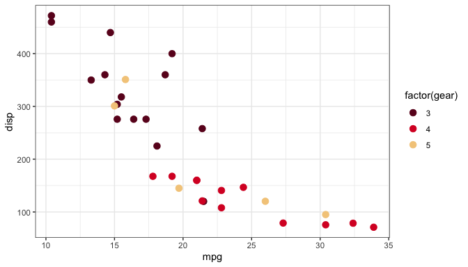
show_palette(omega_nebula)You need to use unname (or use_names=FALSE in read_ase or
read_aco) before using them as values:
library(ggplot2)
gg <- ggplot(mtcars, aes(x=mpg, y=disp))
gg <- gg + geom_point(aes(col=factor(gear)), size=3)
gg <- gg + scale_color_manual(values=unname(keep_the_change))
gg <- gg + theme_bw()
ggPlease note that this project is released with a Contributor Code of Conduct. By participating in this project you agree to abide by its terms.

