Stochastic Simulation of Multiple RPA Binding, Unbinding, Mode Switching and Diffusion on a long ssDNA

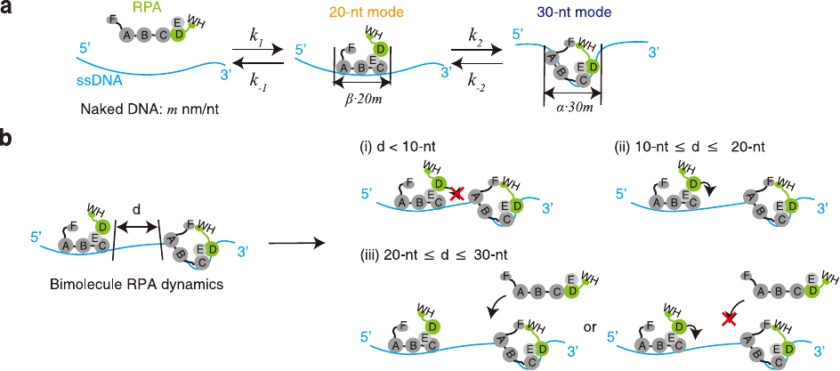
Welcome to our research project on stochastic simulation of multiple RPA binding, unbinding, mode switching, and diffusion on a long ssDNA. In this project, we aim to develop a computational model that can simulate the behavior of RPA (Replication Protein A) molecules on a long single-stranded DNA (ssDNA) molecule, taking into account various stochastic processes such as binding, unbinding, mode switching, and diffusion.

Our model is based on the Tonks-Girardeau gas model, which is a well-known model in statistical physics that describes the behavior of a one-dimensional gas of hard-core bosons. We have extended this model to include the effects of RPA molecules on ssDNA, and have implemented it using the Julia programming language.

For a complete description of our model, please refer to our paper or the simulation_method.

Our simulation results show that our model can accurately capture the behavior of RPA molecules on ssDNA, and can provide insights into the mechanisms underlying RPA-mediated DNA replication and repair. We hope that our work will contribute to a better understanding of these important biological processes, and will inspire further research in this area.

Dependencies

This repository is dependent fully on julialang and its ecosystem. Julia Version 1.8.3 is used in the development of this package. Modules used

CSV v0.10.8
Plots v1.38.0
DataFrames v1.5.0
ProgressMeter v1.7.2
Pipe v1.3.0
Unitful v1.12.2
StatsPlots v0.15.5
Plotly v0.4.1

For complete dependency, see Project.toml and Manifest.toml.

Initialization

Make sure you have julialang and relevant packages installed. Clone this package, and run julia initialize.jl in the command line. This is to precompile the package and generate the folders.

Experiment Data Preparation

The functions for reading experiment data are written in evaluate_base.jl and `evaluate_base_diffusion.jl.

As is mentioned in the paper, we prepare the data by first incubating ssDNA with the RPA for 30 minutes and changed to a higher concentration of RPA later. This is the situation our code is primarily intended to analyze.

Data are stored in the format of csv files. Each csv file consists of a single column of DNA extensions recorded by the ssDNA curtain assay. The first row is ssDNA extension measured at time=5 seconds after flow. The n-th row is ssDNA extension measured at time $5n$ seconds after flow.

1.000000000000000000e+00
1.000000000000000000e+00
1.000000000000000000e+00
1.000000000000000000e+00
1.000000000000000000e+00
1.000000000000000000e+00
1.000000000000000000e+00
1.000000000000000000e+00
...

The data are first grouped by salt, protein concentrations and type of proteins. Each elementary group of data are placed under the same folder. Elementary groups are further grouped together by salt concentration and type of proteins. The secondary groups are a basic set of experiments

The directory tree for the experiment data folder is given as follows.

.
├── data_exp
│   ├── exp_data_lwt0
│   ├── exp_data_lwt1
│   ├── exp_data_lwt10
│   ├── exp_data_lwt25
│   ├── exp_data_lwt4
│   ├── exp_data_lwt50
│   ├── exp_data_wt0
│   ├── exp_data_wt1
│   ├── exp_data_wt10
│   ├── exp_data_wt25
│   ├── exp_data_wt4
│   └── exp_data_wt50

The mapping from folder name to experiment conditions (experiment labels) is stored as a dictionary in the evaluate_base.jl.

    if exp_label == "wt_15mM_salt"
        global exp_data_base=[("wt",0),("wt",1),("wt",4),("wt",10),("wt",25),("wt",50)]
        global folds = [0,1,4,10,25]
    ...
    end
    function salt_concentration(type) 
        if type == "wt"
            return "15mM salt"
        elseif type == "lwt"
            return "150mM salt"
        end
    end
    function exp_dict_inject(type::String,concentration::Float64)
        datapath = "$(mainpath)/data_exp/exp_data_$(type)$(concentration)/"
        fig_label = "$(salt_concentration(type)) yRPA 0.1nM to $(concentration)nM"
        exp_dict["$concentration"]=[datapath,fig_label]
    end
    function exp_dict_inject(type::String,concentration::Int)
        datapath = "$(mainpath)/data_exp/exp_data_$(type)$(concentration)/"
        fig_label = "$(salt_concentration(type)) yRPA 0.1nM to $(concentration)nM"
        exp_dict["$(convert(Float64,concentration))"]=[datapath,fig_label]
    end
    function exp_dict_inject(tuple::Tuple)
        if length(tuple) == 2
            type,concentration = tuple
            exp_dict_inject(type,concentration)
        else
            println("input not match")
        end
    end
    exp_dict_inject.(exp_data_base)

Topology of Codes and Data

Dependency

TonksGaswithReactionGaps.jl -> simu_base.jl -> auto_update.jl/sensitivity_length.jl/sensitivity_diffusion.jl/sensitivity_parameter.jl
evaluate_base.jl -> evaluate.jl/evaluate_sensitivity.jl

A -> B means B depends on A.

Basic Usage

At the root directory, simulation data can be obtained by executing the following command in command line:

julia simu_base.jl $k_on $k_off $v_open $v_close $fold $L $T1 $T2 $N $exp_label $simu_label $gaps_type

where $k_on, $k_off, ..., should be replaced by numerical values. exp_label and simu_label are strings and concatenated to create a unique identifier for the output. $gaps_type can be exact, cumulative or none. It corresponds to different ways of counting the gaps, or not counting them at all.

All the outputs are stored in the folder data_simu/. To generate trace figures, use the following command:

julia evaluate.jl $exp_label $simu_label

This command will combine the simulation and experimentally obtained traces. The code in evaluate.jl could be tailored to custom needs. Accompanying the figures, the code also generates the data source for the figures.

To analyze the gap distribution, use exact_gap_analysis.jl as follows:

julia exact_gap_analysis.jl $exp_label $simu_label

Batch Analysis

auto_update.jl is built on top of the basic analysis method, to automatically find an optimal value of parameters. It relies on the file figs/sources/ini_para.csv to get the initial parameters.

auto_summarize.jl summarizes the data generated by auto_update.jl and the output parameters will be saved in figs/para_$(simu_label).csv The default simu_label for auto_summarize.jl is fitted.

sensitivity_parameter.jl, sensitivity_length.jl, sensitivity_diffusion.jl detect the local sensitivity of the model at the optimal parameter. In those cases, only one parameter is varied and we inspect the losses as a function of this parameter.

chemical_constants.jl estimates some chemical constants based on fitted parameters. The output is saved in figs/sources/kinetics.csv.

Publication

@article{ding2023ssdna,
  title={ssDNA accessibility of Rad51 is regulated by orchestrating multiple RPA dynamics},
  author={Ding, Jiawei and Li, Xiangting and Shen, Jiangchuan and Zhao, Yiling and Zhong, Shuchen and Lai, Luhua and Niu, Hengyao and Qi, Zhi},[^3^][3]
  journal={Nature Communications},
  volume={14},
  number={1},
  pages={3864},
  year={2023},
  doi = {10.1038/s41467-023-39579-y},
  publisher={Nature Publishing Group}
}

hsianktin/RPA_model