No need to install Python or R - your Mac and HiTSEQ-MacOS can provide you results in seconds, complete with data visualization capabilities. Easy to use and lightning fast!
macOS 14.0 (Sonoma)
HiTS-EQ-MacOS app is notarized. For detail, please see Apple's document.
To begin using HiTSEQ on a Mac, download the HiTSEQ-MacOS.zip file and extract its contents. Once unzipped, you'll be able to access and utilize the software without any further steps.
- The csv file does NOT have headers.
- There are 3 columns in your csv file.
- The first column is for random sequence variants. Usually it contains sequences with 6 to 7 nucleotides.
- The second column is for your control point without any binding performed. Just your random library.
- The third column is for your binding point.
- The data type for each column is [String, Integer, Integer]
- For each row, your data may look like:
| AAAAAA | 4329 | 2343 |
|---|---|---|
| AAAAAC | 3452 | 1342 |
| AAAAAG | 2353 | 2342 |
or
| AAAAAAA | 439 | 233 |
|---|---|---|
| AAAAAAC | 345 | 134 |
| AAAAAAG | 233 | 232 |
There is a sample input data for your convenience.
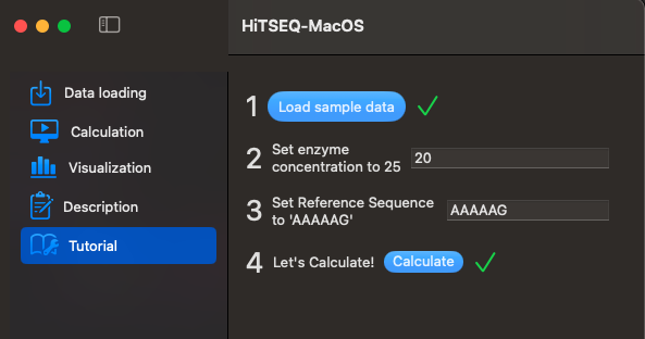
There is also a demo data in this app tutorial part for you to play around.
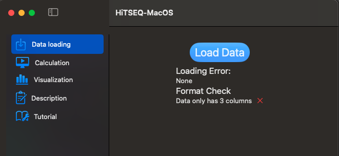
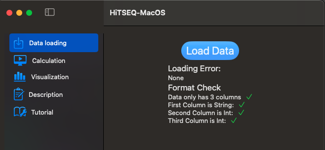
Data loading function will load your csv file and check the format for you.
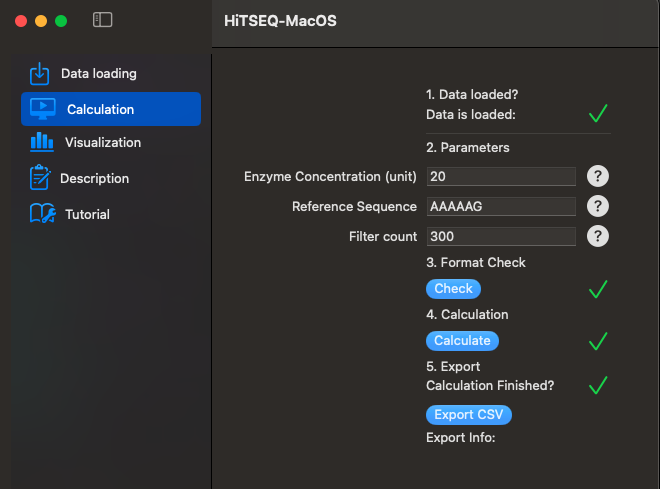
Now we can go to Calculation function. Just follow steps 1 to 5, and you will get your results.
- Enzyme Concentration: It is the concentration of your enzyme/protein/RNA/DNA etc. when you performed the binding experiment for the second column.
- Reference Sequence: The sequence variant you usually use for normalize/compare your results.
- Filter count: When performing sample preparation, there might be issues which cause the sequences can not be amplified well. Those issues may include RT, PCR, or anything. Setting this threshold can help you mark sequences with low reads. Even though the app still calculate and export all sequence variants for you, you can filter them out by the N or Y mark in Excel or any tool.
There will be a column indicate N or Y. N means the reads of the sequence variant in the first column is less than the threshold.
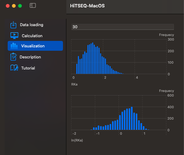
Two histograms are provided for your observation. The difference lies in the x-axis. One represents Relative Rate Constant (RKa), while the other depicts log(RKa). The y-axis, on the other hand, shows Frequency (sequence count).
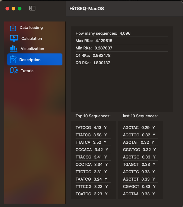
The top 10 sequences and 10 sequences with lowest RKa will be shown here.
A sample dataset is provided for your convenience. Click Load sample data and Calculate to play around.

