Maxwell Austensen (@austensen)
Hayley Raetz (@hayley-raetz)
Jiaqi Dong (@Mocha22ol)
The analysis presented here appears in these two blog posts:
What are the Housing Costs of Households Most Vulnerable to Job Layoffs? An Initial Analysis
COVID-19 and the Rental Market
# Install required packages

# pkgs <- c(
#   "tidyverse",
#   "googlesheets4",
#   "hrbrthemes",
#   "srvyr",
#   "knitr",
#   "rmarkdown",
#   "sf",
#   "dotenv"
# )

# install.packages(pkgs)library(tidyverse) # general data manipulation and graphing
library(googlesheets4) # google sheets
library(srvyr) # survey functions
library(knitr) # markdown table with kable()
library(sf) # spatial data
library(dotenv) # load environment variables from ".env" file
# Load custom functions to help with plotting
source("R/utils.R")
# No scientific notation in outputs
options(scipen = 999)
# Interactively authorize the {googlesheets4} package to access your Google
# account and then cache the authorization token for subsequent uses.
# You must set your google email in the ".env" file (see ".env_sample")
options(
gargle_oauth_email = Sys.getenv("GOOGLE_EMAIL"),
gargle_oauth_cache = ".cache"
)
sheets_auth()To conduct this analysis we used IPUMS occupation code (occ) to
separate occupations into two categories: those with the highest risk of
mass layoffs and workplace closures due to the pandemic; and those
likely to be more protected from widespread disruption. For more
information on our the approach, see our blog post based on this
analysis What are the Housing Costs of Households Most Vulnerable to
Job Layoffs? An Initial
Analysis.
We invite constructive criticism and a dialogue over the methodology for classifying these occupation. You can view and comment on the classification in this Google Sheet, and we look forward to any advice or feedback you might have.
# Read in the occupation risk classification

occ_risk_sheet <- "https://docs.google.com/spreadsheets/d/18dmgZC_sQZOc9AxETwqs7Wc9P6QmCG62y40wlFxXMMk"

occ_risk_xwalk <- occ_risk_sheet %>%
read_sheet(col_types = "ld___", col_names = c("risk_group", "occ"), skip = 1)All data for this analysis comes from IPUMS USA, University of
Minnesota. To build on this analysis and/or
replicate it for a different geography, you can sign up for a free
account and download your own extract of the data. From the IPUMS USA
page, go to Select Data and choose the variables. In addition to to
automatically pre-selected variables, you’ll to select the following
other variables: statefip, countyfip, puma, occ, incwage,
hhincome, ownershp, rentgrs, unitsstr, hispan, and race.
Then click Change Samples to select the data sample you want to use
(for this analysis we have used ACS 2018 1-year). Once you have all your
variables and samples selected, click View Cart and then Create
Extract. The default options here are fine (format: .csv, structure:
Rectangular (person)), and by default you’ll download data for the whole
country. You can click Select Cases, then statefip to export data
for only the states you select. Once the request is complete, download
the file to the /data folder and adjust the following section of code
to reflect your file name and filter to your desired geography.
# Read in IPUMS USA ACS microdata, filter to desired geography

ipums_raw <- read_csv("data/ipums_acs-2018-1yr_ny.csv.gz") %>%
  rename_all(str_to_lower) %>%
  filter(
    # Keep only NYC
    statefip == 36,
    countyfip %in% c(5, 47, 61, 81, 85)
  )
# Create all person- and household-level variables for analysis
ipums_clean <- ipums_raw %>%
filter(
# Remove group quarters population
gq %in% 1:2
) %>%
# Join in risk_group occupation flag
left_join(occ_risk_xwalk, by = "occ") %>%
mutate(
# Set missing values
inc_wages = incwage %>% na_if(999999) %>% na_if(999998) %>% na_if(0),
# There are lots of people with occupation codes but no wages, for this
# analysis we'll count them as not having that occupation, and like people
# without an OCC code will have risk_group=NA
risk_group = if_else(is.na(inc_wages), NA, risk_group),
risk_group_lab = if_else(risk_group, "More vulnerable", "Less vulnerable"),
risk_wages = if_else(risk_group, inc_wages, NA_real_),
# Household income
hh_inc_nom = case_when(
hhincome <= 0 ~ 0,
hhincome == 9999999 ~ NA_real_,
TRUE ~ hhincome
),
hh_inc_grp = cut(
hh_inc_nom, c(-Inf, 15e3, 30e3, 50e3, 75e3, 112.5e3, 150e3, Inf),
c("< $15k", "$15k - 30k", "$30k - $50k", "$50k - $75k", "$75k - $112.5k", "$112.5k - $150k", ">= $150k"),
include.lowest = TRUE,
ordered_result = TRUE
),
# Various renter variables. These are household level variables, and will
# only be used later after filtering to one row per household.
is_renter = (ownershp == 2),
gross_rent_nom = if_else(is_renter, rentgrs, NA_real_),
gross_rent_grp = cut(
gross_rent_nom,
c(-Inf, 600, 1000, 1400, 1800, 2200, Inf),
c("< $600", "$600 - 1,000", "$1,000 - $1,400", "$1,400 - $1,800", "$1,800 - $2,200", ">= $2,200"),
include.lowest = TRUE,
ordered_result = TRUE
),
is_rent_burdened = (rentgrs > (hh_inc_nom / 12 * 0.30)),
is_rent_burdened_sev = (rentgrs > (hh_inc_nom / 12 * 0.50)),
is_rent_burdened_mod = (is_rent_burdened) & (!is_rent_burdened_sev),
# Race/ethnicity labels for graph
race_name = case_when(
hispan %in% 1:4 ~ "Hispanic,\nof any race",
race == 1 ~ "Non-Hispanic\nwhite",
race == 2 ~ "Non-Hispanic\nBlack",
race == 3 ~ "Non-Hispanic\nAmerican\nIndian or\nAlaska Native",
race == 4 ~ "Non-Hispanic\nAsian or\nPacific Islander", # Chinese
race == 5 ~ "Non-Hispanic\nAsian or\nPacific Islander", # Japanese
race == 6 ~ "Non-Hispanic\nAsian or\nPacific Islander", # Other Asian or Pacific Island
race == 7 ~ "Non-Hispanic\nother",
race == 8 ~ "Non-Hispanic\nTwo or more\nmajor races", # Two major races
race == 9 ~ "Non-Hispanic\nTwo or more\nmajor races" # Three or more major races
),
bldg_size = case_when(
unitsstr %in% 3:4 ~ "1",
unitsstr %in% 5:6 ~ "2-4",
unitsstr == 7 ~ "5-9",
unitsstr == 8 ~ "10-19",
unitsstr == 9 ~ "20-49",
unitsstr == 10 ~ "50+",
TRUE ~ "other"
) %>% ordered(levels = c("1","2-4","5-9","10-19","20-49","50+", "other"))
) %>%
# Group by household and categorize households based or occupations of members
group_by(serial) %>%
mutate(
# Household with at least one wage earner in a more vulnerable occupation
# If there are no members with wages then NA, if there are any at-risk
# people with wages then TRUE, if there are people with wages but none of
# them are at risk then FALSE
hh_any_risk = case_when(
all(is.na(risk_group)) ~ NA, # no wage earners
any(risk_group, na.rm = TRUE) ~ TRUE, # any wage earners are at risk
all(!risk_group, na.rm = TRUE) ~ FALSE # all wage earners are at NOT at risk
),
# Household with all wage earners in more vulnerable occupations
# If all members have no wag income then NA, if all the wage earners are in
# the risk group then TRUE, if there are members with wage income but
# none/only some are at risk then FALSE
hh_all_risk = case_when(
all(is.na(risk_group)) ~ NA, # no wage earners
all(risk_group, na.rm = TRUE) ~ TRUE, # all wage earners are at risk
any(!risk_group, na.rm = TRUE) ~ FALSE # not all wage earners are at risk
),
# The total wages for each household that come from vulnerable occupations
hh_risk_wages = sum(risk_wages, na.rm = TRUE),
# The percent of household income that comes from wages from vulnerable occupations
hh_risk_wages_pct = sum(risk_wages, na.rm = TRUE) / na_if(hh_inc_nom, 0)
) %>%
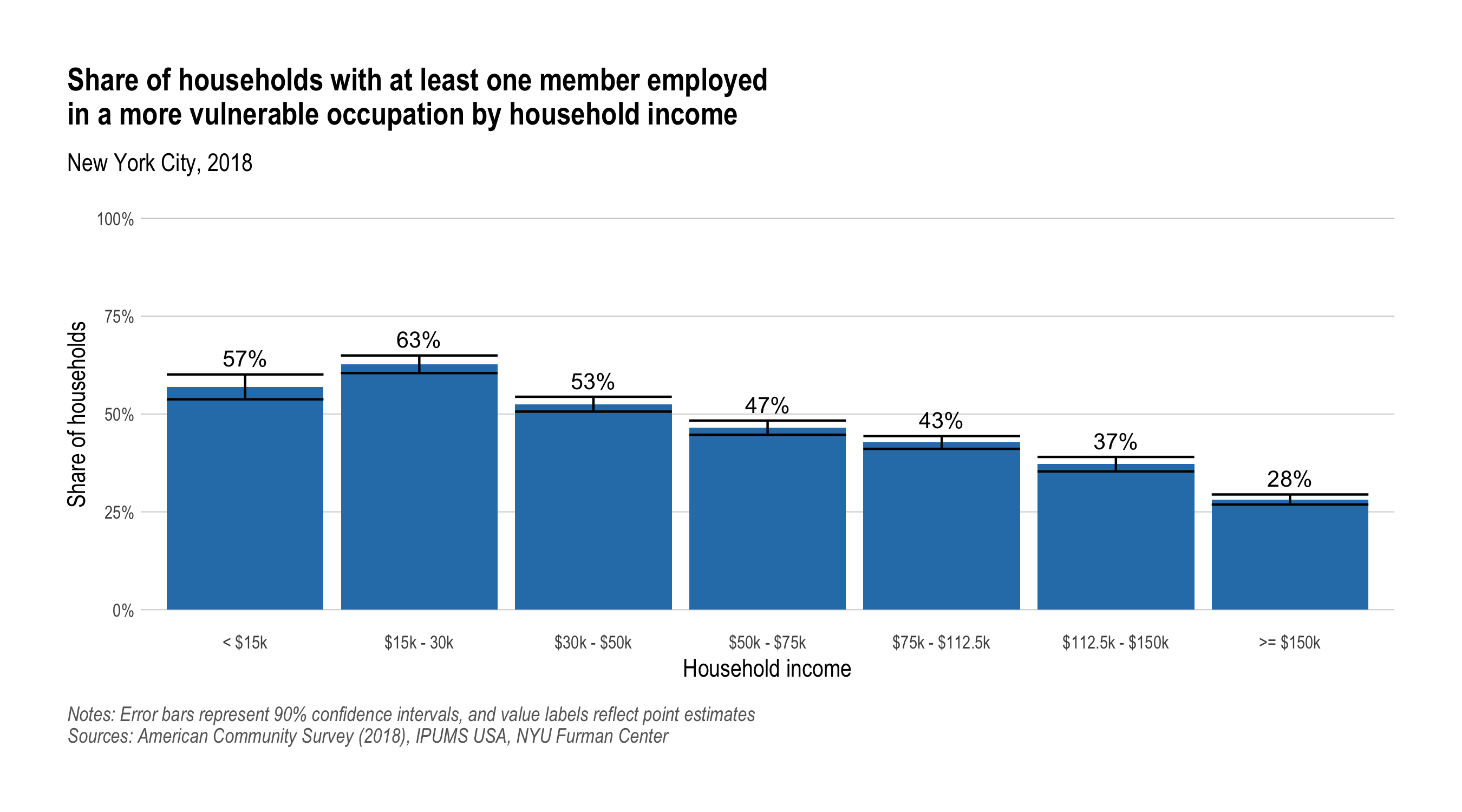
ungroup()# Share of households with at least one member employed in a more vulnerable
# occupation by household income
p <- ipums_clean %>%
filter(
pernum == 1, # keep only one row per household
!is.na(hh_any_risk) # remove households with no wage earners
) %>%
as_survey_design(weights = hhwt) %>%
group_by(hh_inc_grp, .drop = FALSE) %>%
summarise(risk_pct = survey_mean(hh_any_risk, vartype = "ci", level = 0.90)) %>%
ungroup() %>%
fc_col_plot(
x = hh_inc_grp,
y = risk_pct,
ymin = risk_pct_low,
ymax = risk_pct_upp,
y_limits = c(0, 1),
y_format = "percent"
) +
labs(
title = str_glue(
"Share of households with at least one member employed
in a more vulnerable occupation by household income"
),
subtitle = "New York City, 2018",
x = "Household income",
y = str_glue("Share of households"),
caption = str_glue(
"Notes: Error bars represent 90% confidence intervals, and value labels reflect point estimates
Sources: American Community Survey (2018), IPUMS USA, NYU Furman Center"
)
)
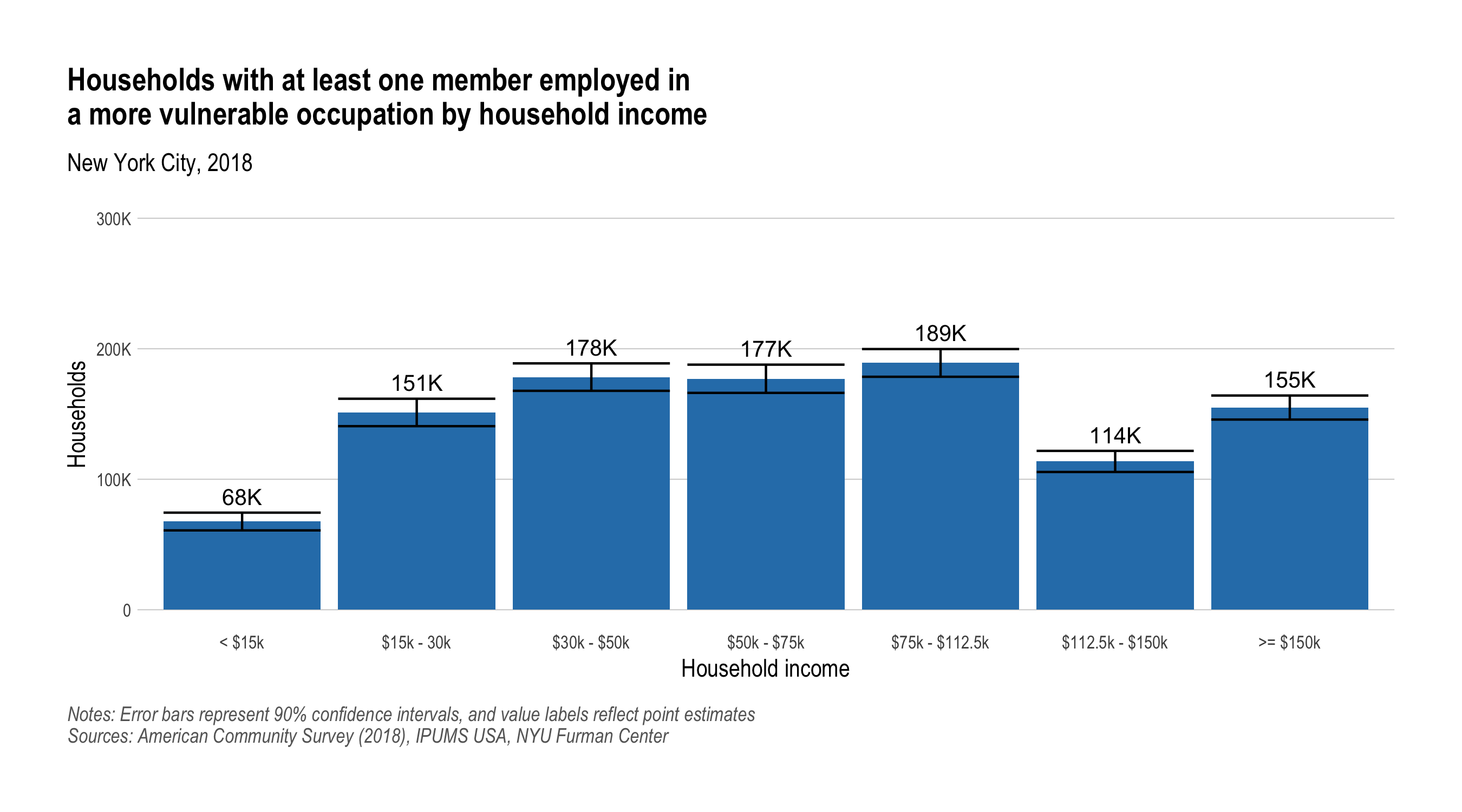
plot_save_include("img/nyc_occ-risk-any_share-income.png")# Households with at least one member employed in a more vulnerable occupation
# by household income
p <- ipums_clean %>%
filter(
pernum == 1, # keep only one row per household
hh_any_risk # keep only households with at least one wage earner in vulnerable occupation
) %>%
as_survey_design(weights = hhwt) %>%
group_by(hh_inc_grp, .drop = FALSE) %>%
summarise(households = survey_total(vartype = "ci", level = 0.90)) %>%
ungroup() %>%
fc_col_plot(
x = hh_inc_grp,
y = households,
y_limits = c(0, 300000),
ymin = households_low,
ymax = households_upp,
y_format = "si"
) +
labs(
title = str_glue(
"Households with at least one member employed in
a more vulnerable occupation by household income"
),
subtitle = "New York City, 2018",
x = "Household income",
y = "Households",
caption = str_glue(
"Notes: Error bars represent 90% confidence intervals, and value labels reflect point estimates
Sources: American Community Survey (2018), IPUMS USA, NYU Furman Center"
)
)
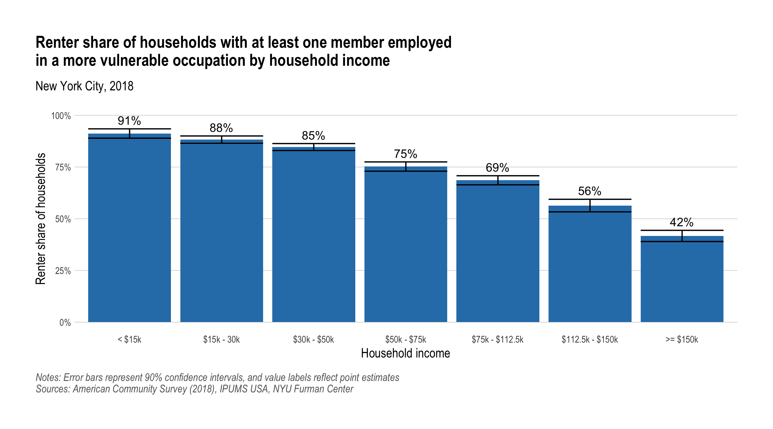
plot_save_include("img/nyc_occ-risk-any_households-income.png")# Renter share of households with at least one member employed in a more
# vulnerable occupation by household income
p <- ipums_clean %>%
filter(
pernum == 1, # keep only one row per household
hh_any_risk # keep only households with at least one wage earner in vulnerable occupation
) %>%
as_survey_design(weights = hhwt) %>%
group_by(hh_inc_grp, .drop = FALSE) %>%
summarise(renter_pct = survey_mean(is_renter, vartype = "ci", level = 0.90)) %>%
ungroup() %>%
fc_col_plot(
x = hh_inc_grp,
y = renter_pct,
y_limits = c(0, 1),
ymin = renter_pct_low,
ymax = renter_pct_upp,
y_format = "percent"
) +
labs(
title = str_glue(
"Renter share of households with at least one member employed
in a more vulnerable occupation by household income"
),
subtitle = "New York City, 2018",
x = "Household income",
y = str_glue("Renter share of households"),
caption = str_glue(
"Notes: Error bars represent 90% confidence intervals, and value labels reflect point estimates
Sources: American Community Survey (2018), IPUMS USA, NYU Furman Center"
)
)
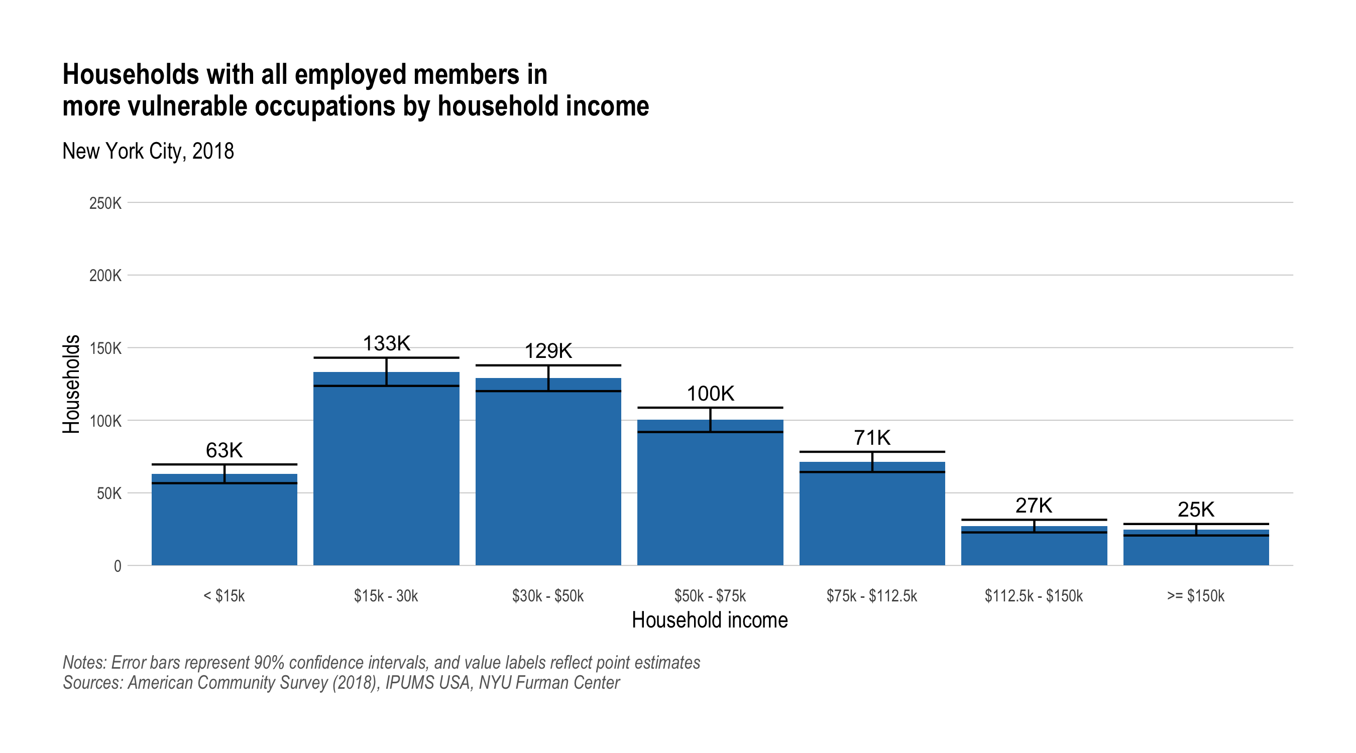
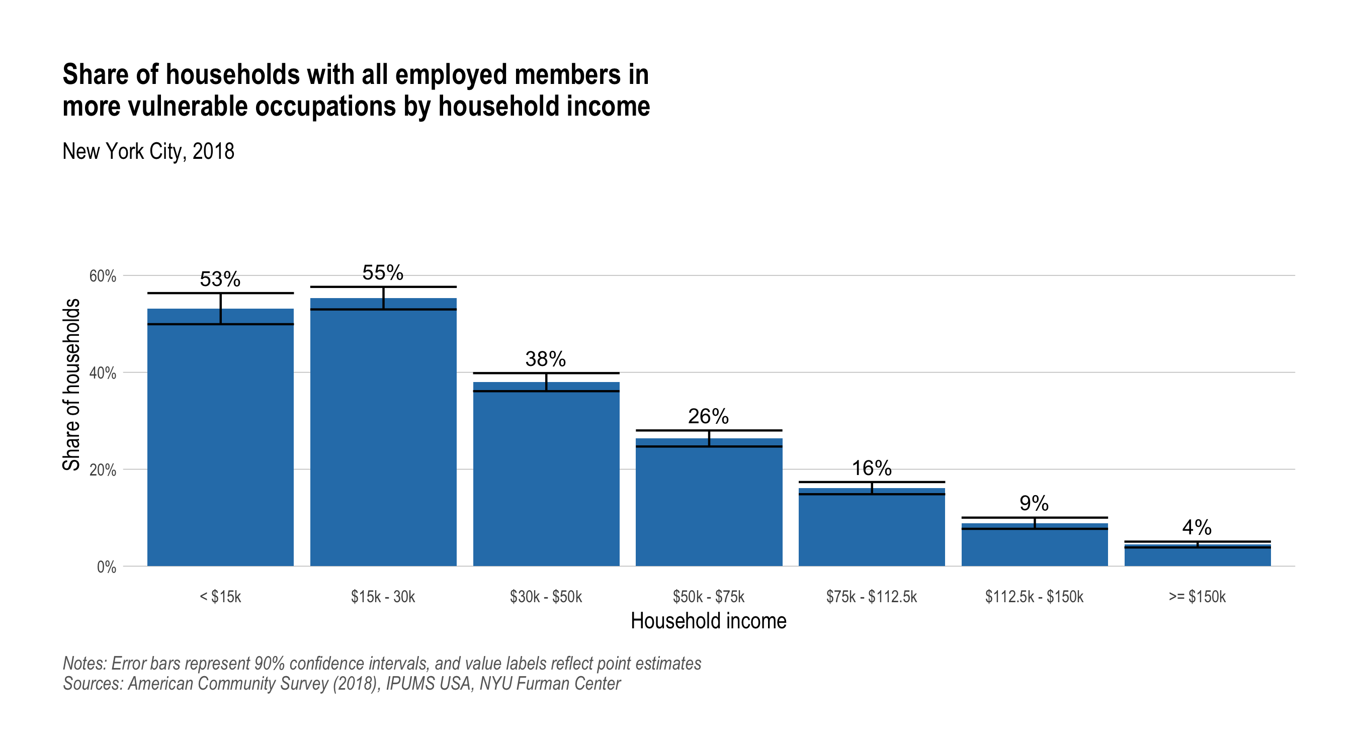
plot_save_include("img/nyc_occ-risk-any_renter-share-income.png")# Households with all employed members in more vulnerable occupations by
# household income
p <- ipums_clean %>%
filter(
pernum == 1, # keep only one row per household
hh_all_risk # keep only households with all wage earners in vulnerable occupations
) %>%
as_survey_design(weights = hhwt) %>%
group_by(hh_inc_grp, .drop = FALSE) %>%
summarise(households = survey_total(vartype = "ci", level = 0.90)) %>%
ungroup() %>%
fc_col_plot(
x = hh_inc_grp,
y = households,
y_limits = c(0, 250000),
ymin = households_low,
ymax = households_upp,
y_format = "si"
) +
labs(
title = str_glue(
"Households with all employed members in
more vulnerable occupations by household income"
),
subtitle = "New York City, 2018",
x = "Household income",
y = "Households",
caption = str_glue(
"Notes: Error bars represent 90% confidence intervals, and value labels reflect point estimates
Sources: American Community Survey (2018), IPUMS USA, NYU Furman Center"
)
)
plot_save_include("img/nyc_occ-risk-all_households-income.png")# Share of households with all employed members in more vulnerable occupations
# by household income
p <- ipums_clean %>%
filter(
pernum == 1, # keep only one row per household
!is.na(hh_all_risk) # keep only households with at least one wage earner
) %>%
as_survey_design(weights = hhwt) %>%
group_by(hh_inc_grp, .drop = FALSE) %>%
summarise(risk_pct = survey_mean(hh_all_risk, vartype = "ci", level = 0.90)) %>%
ungroup() %>%
fc_col_plot(
x = hh_inc_grp,
y = risk_pct,
y_limits = c(0, 0.75),
ymin = risk_pct_low,
ymax = risk_pct_upp,
y_format = "percent"
) +
labs(
title = str_glue(
"Share of households with all employed members in
more vulnerable occupations by household income"
),
subtitle = "New York City, 2018",
x = "Household income",
y = str_glue("Share of households"),
caption = str_glue(
"Notes: Error bars represent 90% confidence intervals, and value labels reflect point estimates
Sources: American Community Survey (2018), IPUMS USA, NYU Furman Center"
)
)
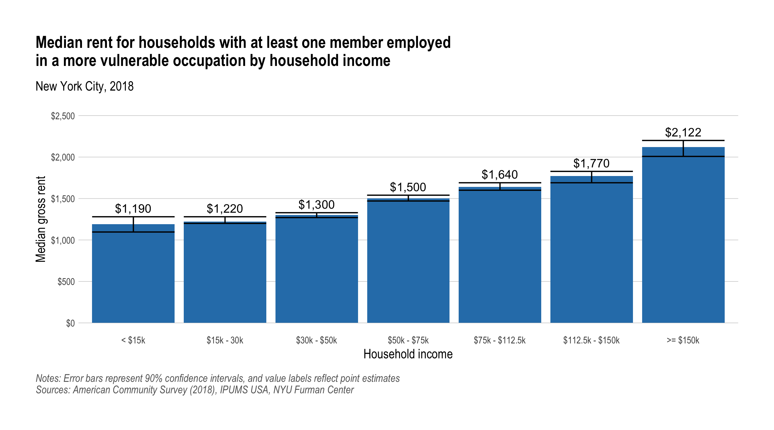
plot_save_include("img/nyc_occ-risk-all_share-income.png")# Median rent for households with at least one member employed in a more
# vulnerable occupation by household income
p <- ipums_clean %>%
filter(
pernum == 1, # keep only one row per household
hh_any_risk, # keep only households with at least one wage earner in vulnerable occupation
is_renter # keep only renter households
) %>%
as_survey_design(weights = hhwt) %>%
group_by(hh_inc_grp, .drop = FALSE) %>%
summarise(gross_rent_nom_med = survey_median(gross_rent_nom, vartype = "ci", level = 0.90)) %>%
ungroup() %>%
fc_col_plot(
x = hh_inc_grp,
y = gross_rent_nom_med,
y_limits = c(0, 2500),
ymin = gross_rent_nom_med_low,
ymax = gross_rent_nom_med_upp,
y_format = "dollar"
) +
labs(
title = str_glue(
"Median rent for households with at least one member employed
in a more vulnerable occupation by household income"
),
subtitle = "New York City, 2018",
x = "Household income",
y = "Median gross rent",
caption = str_glue(
"Notes: Error bars represent 90% confidence intervals, and value labels reflect point estimates
Sources: American Community Survey (2018), IPUMS USA, NYU Furman Center"
)
)
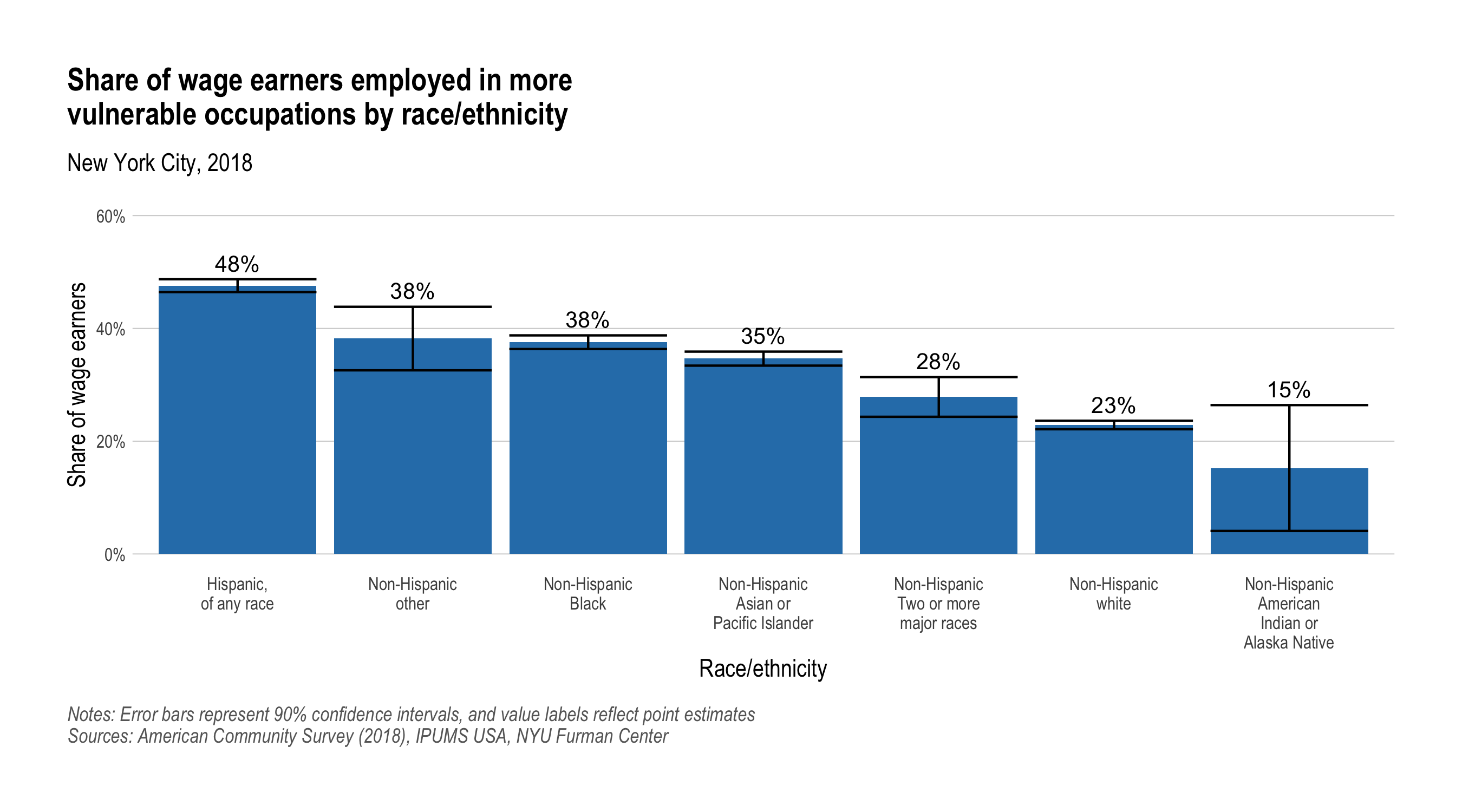
plot_save_include("img/nyc_occ-risk-any_rent-income.png")# Share of wage earners employed in more vulnerable occupations by
# race/ethnicity
p <- ipums_clean %>%
filter(
!is.na(risk_group) # keep only wage earners
) %>%
as_survey_design(weights = perwt) %>%
group_by(race_name, .drop = FALSE) %>%
summarise(pop_pct = survey_mean(risk_group, vartype = "ci", level = 0.90)) %>%
ungroup() %>%
mutate(race_name = fct_reorder(race_name, -pop_pct)) %>%
fc_col_plot(
x = race_name,
y = pop_pct,
y_limits = c(0, 0.6),
ymin = pop_pct_low,
ymax = pop_pct_upp,
y_format = "percent"
) +
labs(
title = str_glue(
"Share of wage earners employed in more
vulnerable occupations by race/ethnicity"
),
subtitle = "New York City, 2018",
x = "Race/ethnicity",
y = str_glue("Share of wage earners"),
caption = str_glue(
"Notes: Error bars represent 90% confidence intervals, and value labels reflect point estimates
Sources: American Community Survey (2018), IPUMS USA, NYU Furman Center"
)
)
plot_save_include("img/nyc_occ-risk_pop-share-race.png")# Create distributions of renter households by building size, for "any risk"
# (more vulnerable) and "no risk" (less vulnerable), including CIs
size_more_vul <- ipums_clean %>%
filter(
pernum == 1, # keep only one row per household
hh_any_risk, # keep only households with at least one wage earner in vulnerable occupation
is_renter #keep only renter households
) %>%
as_survey_design(weights = perwt) %>%
group_by(bldg_size, .drop = FALSE) %>%
summarise(households = survey_total(vartype = "ci", level = 0.90))
total_more_vul <- size_more_vul %>%
mutate(
households_moe = households_upp - households,
households_moe_sqr = households_moe^2
) %>%
summarize(
total = sum(households),
total_moe = sqrt(sum(households_moe_sqr))
)
size_more_vul_rates <- size_more_vul %>%
mutate(
households_moe = households_upp - households,
total = total_more_vul[["total"]],
total_moe = total_more_vul[["total_moe"]],
share = households / total,
share_moe = (1 / total) * sqrt(households_moe^2 - (share * total_moe)^2),
share_low = share - share_moe,
share_upp = share + share_moe
) %>%
select(bldg_size, share, share_low, share_upp) %>%
mutate(category = "More vulnerable")
size_less_vul <- ipums_clean %>%
filter(
pernum == 1, # keep only one row per household
!hh_any_risk, # keep only households without at least one wage earner in vulnerable occupation
is_renter #keep only renter households
) %>%
as_survey_design(weights = perwt) %>%
group_by(bldg_size, .drop = FALSE) %>%
summarise(households = survey_total(vartype = "ci", level = 0.90))
total_less_vul <- size_less_vul %>%
mutate(
households_moe = households_upp - households,
households_moe_sqr = households_moe^2
) %>%
summarize(
total = sum(households),
total_moe = sqrt(sum(households_moe_sqr))
)
size_less_vul_rates <- size_less_vul %>%
mutate(
households_moe = households_upp - households,
total = total_less_vul[["total"]],
total_moe = total_less_vul[["total_moe"]],
share = households / total,
share_moe = (1 / total) * sqrt(households_moe^2 - (share * total_moe)^2),
share_low = share - share_moe,
share_upp = share + share_moe
) %>%
select(bldg_size, share, share_low, share_upp) %>%
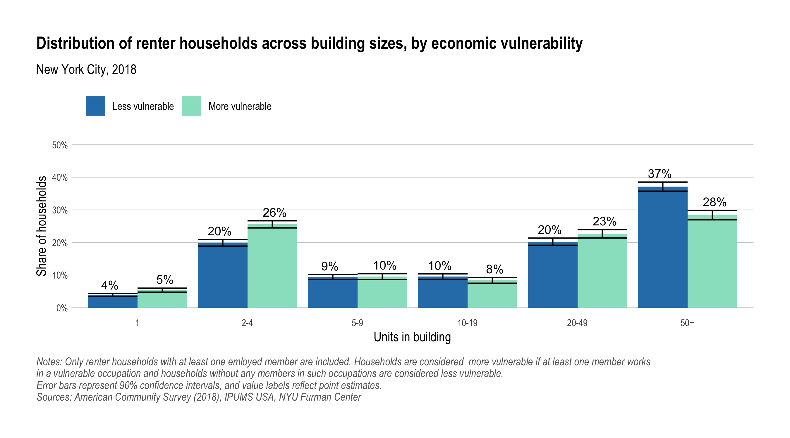
mutate(category = "Less vulnerable")p <- bind_rows(size_less_vul_rates, size_more_vul_rates) %>%
filter(bldg_size != "other") %>%
fc_col_plot_cluster(
x = bldg_size,
y = share,
fill = category,
y_limits = c(0, 0.5),
ymin = share_low,
ymax = share_upp,
y_format = "percent"
) +
scale_fill_manual(values = c("#2c7fb8", "#98e2c9")) +
labs(
title = str_glue(
"Distribution of renter households across building sizes, by economic vulnerability"
),
subtitle = "New York City, 2018",
x = "Units in building",
y = "Share of households",
fill = NULL,
caption = str_glue(
"Notes: Only renter households with at least one emloyed member are included. Households are considered more vulnerable if at least one member works
in a vulnerable occupation and households without any members in such occupations are considered less vulnerable.
Error bars represent 90% confidence intervals, and value labels reflect point estimates.
Sources: American Community Survey (2018), IPUMS USA, NYU Furman Center"
)
)
plot_save_include("img/nyc_renter-risk_bldg_size.png")# Calculate various stats about renter households for the same more and less
# vulnerable groups as above.
more_less_vul_stats <- ipums_clean %>%
filter(
pernum == 1, # keep only one row per household
!is.na(hh_any_risk), # keep only households with at least one wage earner
is_renter # keep only renter households
) %>%
as_survey_design(weights = hhwt) %>%
group_by(hh_any_risk) %>%
summarise(
hh_gross_rent_med = survey_median(gross_rent_nom, vartype = "ci", level = 0.90),
hh_gross_rent = survey_quantile(gross_rent_nom, 0.75, vartype = "ci", level = 0.90),
hh_rent_burdened_pct = survey_mean(is_rent_burdened, vartype = "ci", level = 0.90),
hh_rent_burdened_mod_pct = survey_mean(is_rent_burdened_mod, vartype = "ci", level = 0.90),
hh_rent_burdened_sev_pct = survey_mean(is_rent_burdened_sev, vartype = "ci", level = 0.90)
) %>%
ungroup() %>%
pivot_longer(-hh_any_risk) %>%
mutate(
type = case_when(
str_detect(name, "_low") ~ "low",
str_detect(name, "_upp") ~ "upp",
TRUE ~ "est"
),
name = str_remove(name, "(_low|_upp)"),
hh_any_risk = recode(as.character(hh_any_risk), "TRUE" = "More vulnerable", "FALSE" = "Less vulnerable")
) %>%
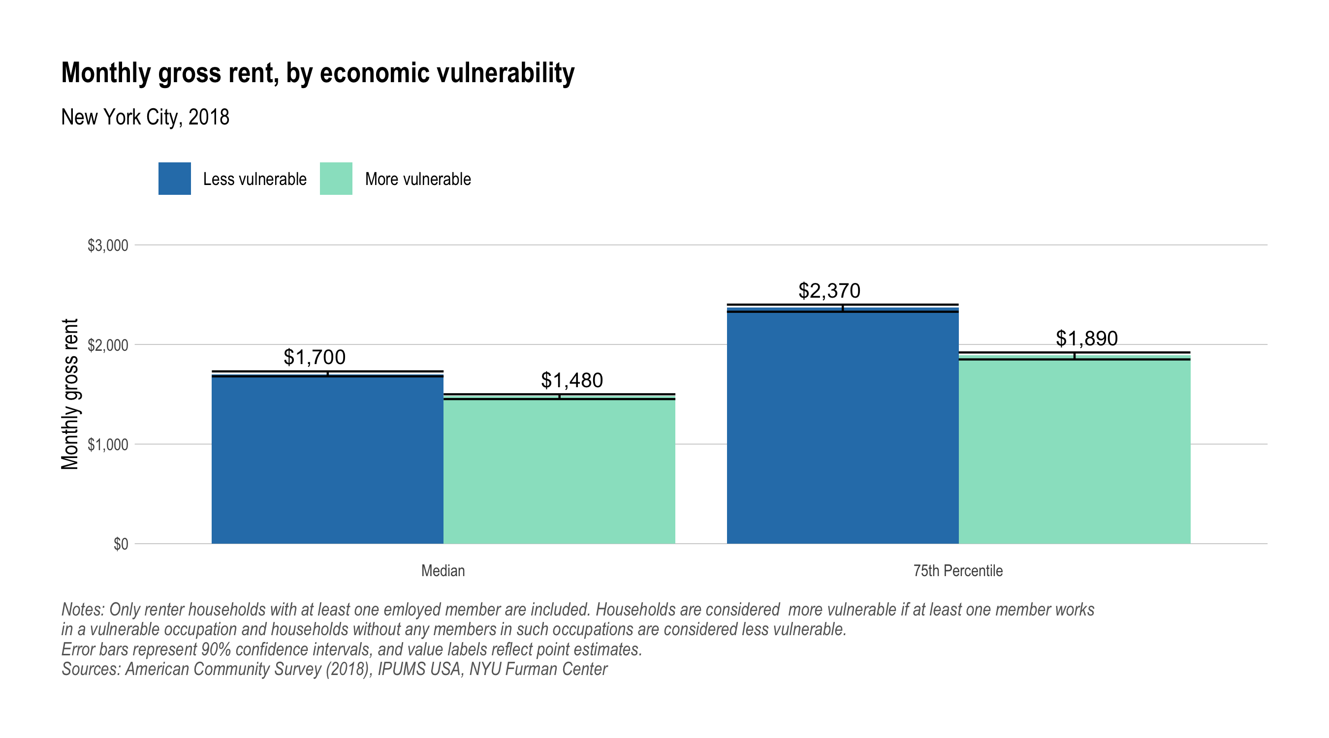
pivot_wider(names_from = type, values_from = value)p <- more_less_vul_stats %>%
filter(str_detect(name, "gross_rent")) %>%
mutate(
name = name %>%
recode("hh_gross_rent_med" = "Median", "hh_gross_rent_q75" = "75th Percentile") %>%
ordered(levels = c("Median", "75th Percentile"))
) %>%
fc_col_plot_cluster(
x = name,
y = est,
fill = hh_any_risk,
y_limits = c(0, 3000),
ymin = low,
ymax = upp,
y_format = "dollar"
) +
scale_fill_manual(values = c("#2c7fb8", "#98e2c9")) +
labs(
title = str_glue(
"Monthly gross rent, by economic vulnerability"
),
subtitle = "New York City, 2018",
x = NULL,
y = "Monthly gross rent",
fill = NULL,
caption = str_glue(
"Notes: Only renter households with at least one emloyed member are included. Households are considered more vulnerable if at least one member works
in a vulnerable occupation and households without any members in such occupations are considered less vulnerable.
Error bars represent 90% confidence intervals, and value labels reflect point estimates.
Sources: American Community Survey (2018), IPUMS USA, NYU Furman Center"
)
)
plot_save_include("img/nyc_renter-risk_gross-rent.png")p <- more_less_vul_stats %>%
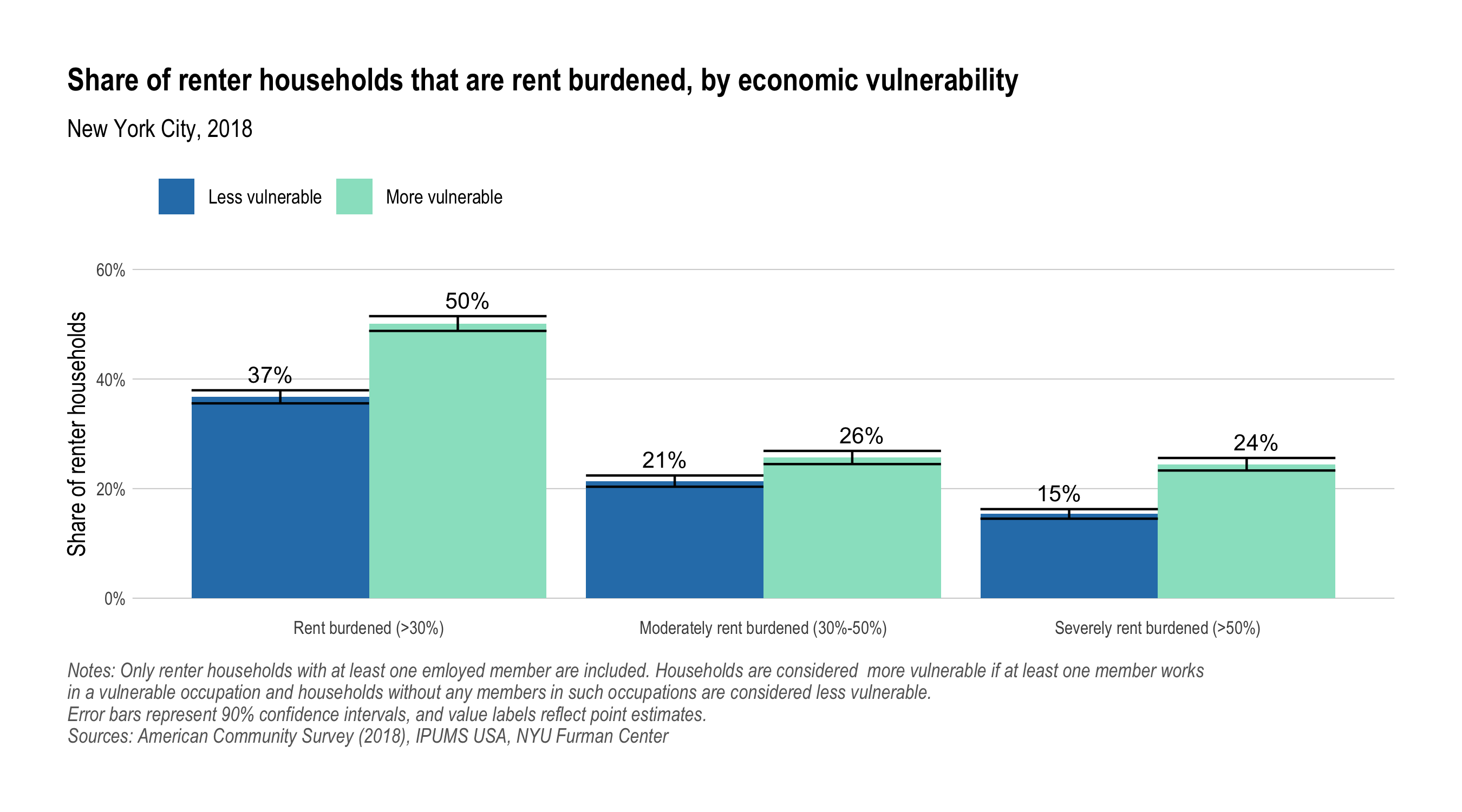
filter(str_detect(name, "burden")) %>%
mutate(
name = name %>%
recode("hh_rent_burdened_pct" = "Rent burdened (>30%)",
"hh_rent_burdened_mod_pct" = "Moderately rent burdened (30%-50%)",
"hh_rent_burdened_sev_pct" = "Severely rent burdened (>50%)") %>%
ordered(levels = c("Rent burdened (>30%)", "Moderately rent burdened (30%-50%)", "Severely rent burdened (>50%)"))
) %>%
fc_col_plot_cluster(
x = name,
y = est,
fill = hh_any_risk,
y_limits = c(0, 0.6),
ymin = low,
ymax = upp,
y_format = "percent"
) +
scale_fill_manual(values = c("#2c7fb8", "#98e2c9")) +
labs(
title = str_glue(
"Share of renter households that are rent burdened, by economic vulnerability"
),
subtitle = "New York City, 2018",
x = NULL,
y = "Share of renter households",
fill = NULL,
caption = str_glue(
"Notes: Only renter households with at least one emloyed member are included. Households are considered more vulnerable if at least one member works
in a vulnerable occupation and households without any members in such occupations are considered less vulnerable.
Error bars represent 90% confidence intervals, and value labels reflect point estimates.
Sources: American Community Survey (2018), IPUMS USA, NYU Furman Center"
)
)
plot_save_include("img/nyc_renter-risk_rent-burden.png")To map the results of this analysis at the neighborhood level, the first step is to prepare the geomoetries for Public Use Microdata Areas (PUMAs). For New York City the city has a dataset of PUMAs already nicely clipped to the shoreline, for here we’ll be using those and joining on the neighborhood names.
# Get NYC PUMAs from NYC Open Data, and attach local neighborhood names

nyc_puma_names <- read_csv("data/nyc_puma_names.csv")

nyc_pumas_url <- "https://data.cityofnewyork.us/api/geospatial/cwiz-gcty?method=export&format=GeoJSON"
nyc_pumas <- read_sf(nyc_pumas_url) %>%
  transmute(puma = as.numeric(puma)) %>%
  st_transform(2263) %>% # local state plane projection for NYC
  st_simplify(dTolerance = 100) # reduce the detail of the polygons
Elsewhere in the country the best option for getting the geomoetries is
to use the tigris R package to
download Tiger/Line shapefiles from the US Census Bureau.
# {NOT RUN}
# Example of getting PUMA geometries using tirgis package.
library(tigris)

# Easiest option will be to get all PUMAs in the state, then innner join to the NYC IPUMS data
ny_pumas <- tigris::pumas("NY", class = "sf") %>%
  transmute(
    statefip = STATEFP10,
    puma = as.numeric(PUMACE10),
    puma_name = NAMELSAD10
  )
# Set some of the options once here to recude repetition below
survey_mean_ci90 <- purrr::partial(survey_mean, vartype = "ci", level = 0.90)
ipums_puma <- ipums_clean %>%
filter(
pernum == 1, # keep only one row per household
# is_renter, # keep only renter households
!is.na(hh_any_risk) # remove households with no wage earners
) %>%
as_survey_design(weights = hhwt) %>%
# In NYC pumas nest within county, so helpful to keep county/borough IDs
group_by(countyfip, puma) %>%
summarise(
hh_any_risk_renter_pct = survey_mean_ci90(hh_any_risk*na_if(is_renter, FALSE), na.rm = TRUE),
hh_all_risk_renter_pct = survey_mean_ci90(hh_any_risk*na_if(is_renter, FALSE), na.rm = TRUE),
hh_any_risk_pct = survey_mean_ci90(hh_any_risk),
hh_all_risk_pct = survey_mean_ci90(hh_any_risk),
) %>%
ungroup() %>%
mutate(
hh_any_risk_pct_moe = hh_any_risk_pct_upp - hh_any_risk_pct,
hh_anll_risk_pct_moe = hh_all_risk_pct_upp - hh_all_risk_pct,
hh_any_risk_renter_pct_moe = hh_any_risk_renter_pct_upp - hh_any_risk_renter_pct,
hh_anll_risk_renter_pct_moe = hh_all_risk_renter_pct_upp - hh_all_risk_renter_pct,
# Suppress the most unreliable observations, then bin for map
# See notes below about using reliability claculator to decide on these bins
hh_any_risk_renter_pct_grp = ifelse(hh_any_risk_renter_pct_moe > 0.07, NA_real_, hh_any_risk_renter_pct) %>%
cut(
breaks = c(-Inf, 0.4, 0.6, Inf),
labels = c("< 40%", "40% - 60%", ">= 60%"),
include.lowest = TRUE,
ordered_result = TRUE
) %>%
fct_explicit_na("Insufficient Data")
) %>%
select(-matches(".*_(upp|low)$")) %>%
left_join(nyc_pumas, by = "puma") %>%
left_join(nyc_puma_names, by = "puma") %>%
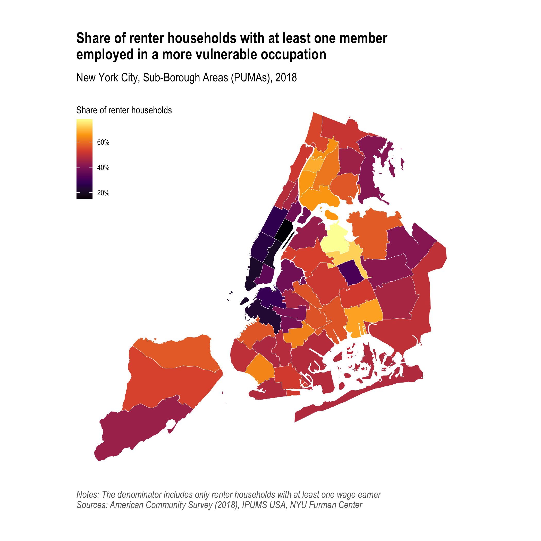
st_as_sf() # dataframe takes class of left table, so change back to spatial typep <- ggplot(ipums_puma) +
aes(fill = hh_any_risk_renter_pct) +
geom_sf(size = 0.1, color = "white") +
scale_fill_viridis_c(labels = scales::percent_format(1), option = "inferno") +
theme_fc_map() +
theme( # some NYC specific tweaks
legend.position = c(0, .85),
legend.direction = "vertical",
legend.margin = margin(0, 0, 0, 0)
) +
labs(
title = str_glue(
"Share of renter households with at least one member
employed in a more vulnerable occupation"
),
subtitle = "New York City, Sub-Borough Areas (PUMAs), 2018",
fill = "Share of renter households",
caption = str_glue(
"Notes: The denominator includes only renter households with at least one wage earner
Sources: American Community Survey (2018), IPUMS USA, NYU Furman Center"
)
)
plot_save_include("img/nyc_occ-risk-any-renter_share-map.png", height = 7, width = 7)The above map doesn’t take in account the reliability of the estimates.
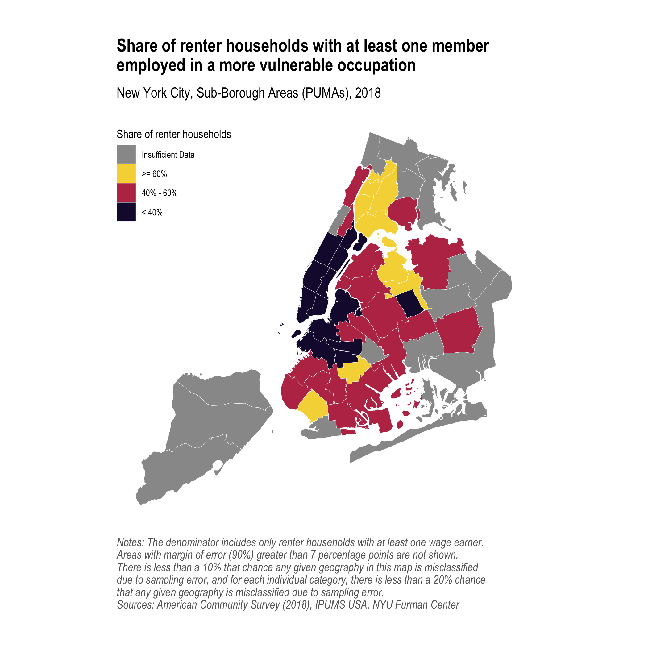
Below the Sub Borough Areas (PUMAs) are categorized into three bins and
pumas with the most unreliable estimates (90% MOE > 7 percentage
points) are suppressed. These categories were selected with the help of
the R package
mapreliability and the
interactive tool
reliability_calculator()
to ensure that there is an acceptable level of potential
missclassification as a result of sampling error. With this
classification, and the most unreliable estimate excluded, there is less
than a 10% that chance any given geography in this map is misclassified
due to sampling error, and for each individual category, there is less
than a 20% chance that any given geography is misclassified due to
sampling
error.
library(mapreliability) # remotes::install_github("austensen/mapreliability")

ipums_puma %>%
  filter(hh_any_risk_renter_pct_moe <= 0.07) %>%
  reliability_table_custom(hh_any_risk_renter_pct, hh_any_risk_renter_pct_moe, c(0, 0.4, 0.6))
## # A tibble: 3 x 5
## class_breaks count tot_count reliability tot_reliability
## <dbl> <int> <int> <dbl> <dbl>
## 1 0 13 40 11.6 9.61
## 2 0.4 18 40 7.51 9.61
## 3 0.6 9 40 10.9 9.61
p <- ggplot(ipums_puma) +
  aes(fill = hh_any_risk_renter_pct_grp) +
  geom_sf(size = 0.1, color = "white") +
  scale_fill_manual(
    values = c(viridisLite::inferno(3, begin = 0.1, end = 0.9), "grey60"),
    guide = guide_legend(reverse = TRUE)
  ) +
  # scale_fill_viridis_d(guide = guide_legend(reverse = TRUE)) +
  theme_fc_map() +
  theme( # some NYC specific tweaks
    legend.position = c(0, .85),
    legend.direction = "vertical",
    legend.margin = margin(0, 0, 0, 0)
  ) +
  labs(
    title = str_glue(
      "Share of renter households with at least one member
      employed in a more vulnerable occupation"
    ),
    subtitle = "New York City, Sub-Borough Areas (PUMAs), 2018",
    fill = "Share of renter households",
    caption = str_glue(
      "Notes: The denominator includes only renter households with at least one wage earner.
      Areas with margin of error (90%) greater than 7 percentage points are not shown.
      There is less than a 10% that chance any given geography in this map is misclassified
      due to sampling error, and for each individual category, there is less than a 20% chance
      that any given geography is misclassified due to sampling error.
      Sources: American Community Survey (2018), IPUMS USA, NYU Furman Center"
    )
  )

plot_save_include("img/nyc_occ-risk-any-renter_share-grp-map.png", height = 7, width = 7)# Total number of households
hh_total <- ipums_clean %>%
filter(
pernum == 1, # keep only one row per household
) %>%
as_survey_design(weights = hhwt) %>%
summarise(
households = survey_total(1, vartype = "ci", level = 0.90)
)
hh_total %>%
pivot_longer(everything()) %>%
kable()| name | value |
|---|---|
| households | 3184458 |
| households_low | 3161148 |
| households_upp | 3207768 |
# Total number of wage earners
wage_earners_total <- ipums_clean %>%
  filter(inc_wages >=0) %>%
  as_survey_design(weights = perwt) %>%
  summarise(
    individuals = survey_total(1, vartype = "ci", level = 0.90)
  )

wage_earners_total %>%
  pivot_longer(everything()) %>%
kable()| name | value |
|---|---|
| individuals | 4085333 |
| individuals_low | 4058659 |
| individuals_upp | 4112007 |
# Population living in households with at least one wage earner in more vulnerable occupation
pop_hh_risk_any <- ipums_clean %>%
  filter(hh_any_risk) %>%
  as_survey_design(weights = perwt) %>%
  summarise(
    individuals = survey_total(1, vartype = "ci", level = 0.90)
  )

pop_hh_risk_any %>%
  pivot_longer(everything()) %>%
kable()| name | value |
|---|---|
| individuals | 3496121 |
| individuals_low | 3471727 |
| individuals_upp | 3520515 |
# Various stats for households with at least one wage earner in vulnerable occupation
hh_any_risk_stats <- ipums_clean %>%
  filter(
    pernum == 1, # keep only one row per household
    hh_any_risk # keep only households with at least one wage earner in vulnerable occupation
  ) %>%
  as_survey_design(weights = hhwt) %>%
  summarise(
    households = survey_total(1, vartype = "ci", level = 0.90),
    hh_inc_nom_med = survey_median(hh_inc_nom, na.rm = TRUE),
    hh_risk_wages_med = survey_median(hh_risk_wages, na.rm = TRUE),
    hh_risk_wages_pct_med = survey_median(hh_risk_wages_pct, na.rm = TRUE),
    gross_rent_nom_med = survey_median(gross_rent_nom, vartype = "ci", na.rm = TRUE)
  )

hh_any_risk_stats %>%
  pivot_longer(everything()) %>%
kable()| name | value |
|---|---|
| households | 1031873.0000000 |
| households_low | 1018905.6246131 |
| households_upp | 1044840.3753869 |
| hh_inc_nom_med | 66589.2401216 |
| hh_inc_nom_med_se | 1021.3159191 |
| hh_risk_wages_med | 33292.9347826 |
| hh_risk_wages_med_se | 765.2109373 |
| hh_risk_wages_pct_med | 0.6511628 |
| hh_risk_wages_pct_med_se | 0.0095706 |
| gross_rent_nom_med | 1480.0000000 |
| gross_rent_nom_med_low | 1450.0000000 |
| gross_rent_nom_med_upp | 1500.0000000 |
# Various stats for households with all wage earners in vulnerable occupations
hh_all_risk_stats <- ipums_clean %>%
  filter(
    pernum == 1, # keep only one row per household
    hh_all_risk # keep only households with all wage earners in vulnerable occupations
  ) %>%
  as_survey_design(weights = hhwt) %>%
  summarise(
    households = survey_total(1, vartype = "ci", level = 0.90),
    hh_inc_nom_med = survey_median(hh_inc_nom, na.rm = TRUE),
    hh_risk_wages_med = survey_median(hh_risk_wages, na.rm = TRUE),
    hh_risk_wages_pct_med = survey_median(hh_risk_wages_pct, na.rm = TRUE),
    gross_rent_nom_med = survey_median(gross_rent_nom, vartype = "ci", na.rm = TRUE)
  )

hh_all_risk_stats %>%
  pivot_longer(everything()) %>%
kable()| name | value |
|---|---|
| households | 548652.0000 |
| households_low | 538877.9518 |
| households_upp | 558426.0482 |
| hh_inc_nom_med | 41200.0000 |
| hh_inc_nom_med_se | 969.1174 |
| hh_risk_wages_med | 33757.1429 |
| hh_risk_wages_med_se | 765.0927 |
| hh_risk_wages_pct_med | 1.0000 |
| hh_risk_wages_pct_med_se | 0.0000 |
| gross_rent_nom_med | 1350.0000 |
| gross_rent_nom_med_low | 1310.0000 |
| gross_rent_nom_med_upp | 1387.1656 |
# Various stats for households making less than $150k and with at least one wage
# earner in a more vulnerable occupation
hh_any_risk_lt150k <- ipums_clean %>%
  filter(
    pernum == 1, # keep only one row per household
    hh_any_risk,
    hh_inc_nom <150000
  ) %>%
  as_survey_design(weights = hhwt) %>%
  summarise(
    households = survey_total(1, vartype = "ci", level = 0.90),
    hh_inc_nom_med = survey_median(hh_inc_nom, na.rm = TRUE),
    hh_risk_wages_med = survey_median(hh_risk_wages, na.rm = TRUE),
    hh_risk_wages_pct_med = survey_median(hh_risk_wages_pct, na.rm = TRUE),
    gross_rent_nom_med = survey_median(gross_rent_nom, na.rm = TRUE)
  )

hh_any_risk_lt150k %>%
  pivot_longer(everything()) %>%
kable()| name | value |
|---|---|
| households | 872156.0000000 |
| households_low | 860239.8717704 |
| households_upp | 884072.1282296 |
| hh_inc_nom_med | 55000.0000000 |
| hh_inc_nom_med_se | 850.8103283 |
| hh_risk_wages_med | 30000.0000000 |
| hh_risk_wages_med_se | 0.0000000 |
| hh_risk_wages_pct_med | 0.7319793 |
| hh_risk_wages_pct_med_se | 0.0140094 |
| gross_rent_nom_med | 1430.0000000 |
| gross_rent_nom_med_se | 15.3025870 |
# Various stats for households making less than $150k and with all wage earners
# in a more vulnerable occupation
hh_all_risk_lt150k <- ipums_clean %>%
  filter(
    pernum == 1, # keep only one row per household
    hh_all_risk,
    hh_inc_nom <150000
  ) %>%
  as_survey_design(weights = hhwt) %>%
  summarise(
    households = survey_total(1, vartype = "ci", level = 0.90),
    hh_inc_nom_med = survey_median(hh_inc_nom, na.rm = TRUE),
    hh_risk_wages_med = survey_median(hh_risk_wages, na.rm = TRUE),
    hh_risk_wages_pct_med = survey_median(hh_risk_wages_pct, na.rm = TRUE),
    gross_rent_nom_med = survey_median(gross_rent_nom, na.rm = TRUE)
  )

hh_all_risk_lt150k %>%
  pivot_longer(everything()) %>%
kable()| name | value |
|---|---|
| households | 521588.00000 |
| households_low | 512056.84270 |
| households_upp | 531119.15730 |
| hh_inc_nom_med | 40000.00000 |
| hh_inc_nom_med_se | 518.39144 |
| hh_risk_wages_med | 31700.00000 |
| hh_risk_wages_med_se | 816.08389 |
| hh_risk_wages_pct_med | 1.00000 |
| hh_risk_wages_pct_med_se | 0.00000 |
| gross_rent_nom_med | 1330.00000 |
| gross_rent_nom_med_se | 17.85005 |
