
| Documentation | Build Status (CPU, GPU, Windows, Docker) | Code coverage |
|---|---|---|
   |
Oceananigans.jl is a fast and friendly incompressible fluid flow solver written in Julia that can be run in 1-3 dimensions on CPUs and GPUs. It is designed to solve the rotating Boussinesq equations used in non-hydrostatic ocean modeling but can be used to solve for any incompressible flow.
Our goal is to develop a friendly and intuitive package allowing users to focus on the science. Thanks to high-level, zero-cost abstractions that the Julia programming language makes possible, the model can have the same look and feel no matter the dimension or grid of the underlying simulation, and the same code is shared between the CPU and GPU.
- Ali Ramadhan (@ali-ramadhan)
- Chris Hill (@christophernhill)
- Jean-Michel Campin (@jm-c)
- John Marshall (@johncmarshall54)
- Greg Wagner (@glwagner)
- Andre Souza (@sandreza)
- James Schloss (@leios)
- Mukund Gupta (@mukund-gupta)
- Zhen Wu (@zhenwu0728)
- On the Julia side, big thanks to Valentin Churavy (@vchuravy), Tim Besard (@maleadt) and Peter Ahrens (@peterahrens)!
You can install the latest stable version of Oceananigans using the built-in package manager (accessed by pressing ] in the Julia command prompt)
julia>]
(v1.1) pkg> add OceananigansNote: Oceananigans requires the latest version of Julia (1.1) to run correctly.
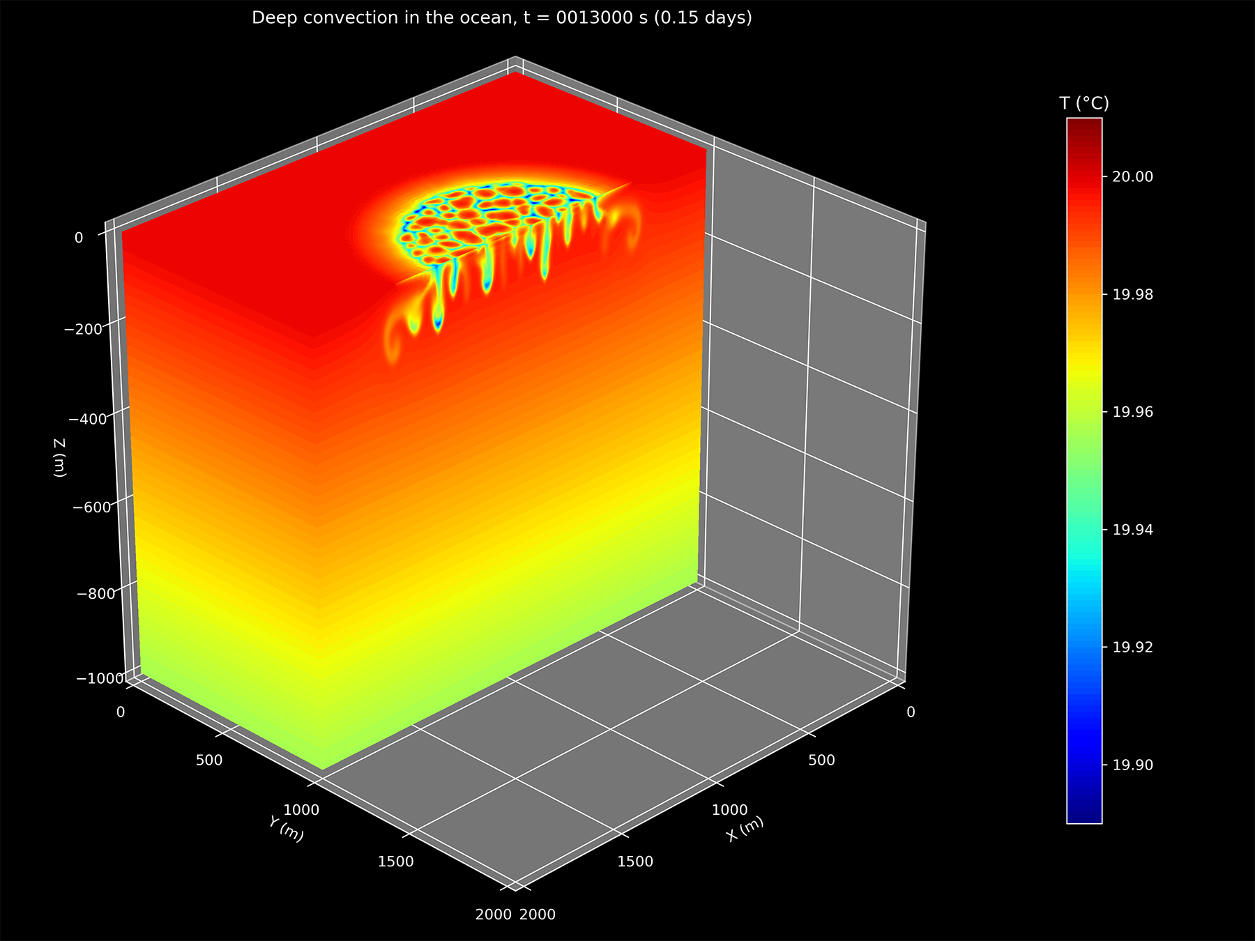
Let's initialize a 3D model with 100×100×50 grid points on a 2×2×1 km domain and simulate it for 10 time steps using steps of 60 seconds each (for a total of 10 minutes of simulation time).
using Oceananigans
model = Model(N=(100, 100, 50), L=(2000, 2000, 1000))
time_step!(model; Δt=60, Nt=10)
You just simulated what might have been a 3D patch of ocean, it's that easy! It was a still lifeless ocean so nothing interesting happened but now you can add interesting dynamics and visualize the output.
Let's add something to make the dynamics a bit more interesting. We can add a hot bubble in the middle of the domain and watch it rise to the surface. This example shows how to set an initial condition.
using Oceananigans

# We'll set up a 2D model with an xz-slice so there's only 1 grid point in y
# and use an artificially high viscosity ν and diffusivity κ.
model = Model(N=(256, 1, 256), L=(2000, 1, 2000), arch=CPU(), ν=4e-2, κ=4e-2)

# Set a temperature perturbation with a Gaussian profile located at the center
# of the vertical slice. This will create a buoyant thermal bubble that will
# rise with time.
Lx, Lz = model.grid.Lx, model.grid.Lz
x₀, z₀ = Lx/2, Lz/2
T₀(x, y, z) = 20 + 0.01 * exp(-100 * ((x - x₀)^2 + (z - z₀)^2) / (Lx^2 + Lz^2))
set!(model; T=T₀)

time_step!(model; Δt=10, Nt=5000)
By changing arch=CPU() to arch=GPU(), the example will run on an Nvidia GPU!
Check out rising_thermal_bubble_2d.jl to see how you can plot a 2D movie with the output.
Note: You need to have Plots.jl and ffmpeg installed for the movie to be automatically created by Plots.jl.
GPU model output can be plotted on-the-fly and animated using Makie.jl! This NextJournal notebook has an example. Thanks @SimonDanisch! Some Makie.jl isosurfaces from a rising spherical thermal bubble (the GPU example):

You can see some movies from GPU simulations below along with CPU and GPU performance benchmarks.
If you are interested in using Oceananigans.jl or are trying to figure out how to use it, please feel free to ask us questions and get in touch! Check out the examples and open an issue if you have any questions, comments, suggestions, etc.
We've performed some preliminary performance benchmarks (see the benchmarks.jl file) by initializing models of various sizes and measuring the wall clock time taken per model iteration (or time step). The CPU used was a single core of an Intel Xeon CPU E5-2680 v4 @ 2.40GHz while the GPU used was an Nvidia Tesla V100-SXM2-16GB. This isn't really a fair comparison as we haven't parallelized across all the CPU's cores so we will revisit these benchmarks once Oceananigans.jl can run on multiple CPUs and GPUs.
